---
bibliography: ref.bib
---
# (PART) Workflows {-}
# H3K9ac, pro-B versus mature B
## Overview
Here, we perform a window-based differential binding (DB) analysis to identify regions of differential H3K9ac enrichment between pro-B and mature B cells [@domingo2012].
H3K9ac is associated with active promoters and tends to exhibit relatively narrow regions of enrichment relative to other marks such as H3K27me3.
For this study, the experimental design contains two biological replicates for each of the two cell types.
We download the BAM files using the relevant function from the *[chipseqDBData](https://bioconductor.org/packages/3.18/chipseqDBData)* package.
```r
library(chipseqDBData)
acdata <- H3K9acData()
acdata
```
```
## DataFrame with 4 rows and 3 columns
## Name Description Path
##
## 1 h3k9ac-proB-8113 pro-B H3K9ac (8113)
## 2 h3k9ac-proB-8108 pro-B H3K9ac (8108)
## 3 h3k9ac-matureB-8059 mature B H3K9ac (8059)
## 4 h3k9ac-matureB-8086 mature B H3K9ac (8086)
```
## Pre-processing checks
### Examining mapping statistics
We use methods from the *[Rsamtools](https://bioconductor.org/packages/3.18/Rsamtools)* package to compute some mapping statistics for each BAM file.
Ideally, the proportion of mapped reads should be high (70-80% or higher),
while the proportion of marked reads should be low (generally below 20%).
```r
library(Rsamtools)
diagnostics <- list()
for (b in seq_along(acdata$Path)) {
bam <- acdata$Path[[b]]
total <- countBam(bam)$records
mapped <- countBam(bam, param=ScanBamParam(
flag=scanBamFlag(isUnmapped=FALSE)))$records
marked <- countBam(bam, param=ScanBamParam(
flag=scanBamFlag(isUnmapped=FALSE, isDuplicate=TRUE)))$records
diagnostics[[b]] <- c(Total=total, Mapped=mapped, Marked=marked)
}
diag.stats <- data.frame(do.call(rbind, diagnostics))
rownames(diag.stats) <- acdata$Name
diag.stats$Prop.mapped <- diag.stats$Mapped/diag.stats$Total*100
diag.stats$Prop.marked <- diag.stats$Marked/diag.stats$Mapped*100
diag.stats
```
```
## Total Mapped Marked Prop.mapped Prop.marked
## h3k9ac-proB-8113 10724526 8832006 434884 82.35 4.924
## h3k9ac-proB-8108 10413135 7793913 252271 74.85 3.237
## h3k9ac-matureB-8059 16675372 4670364 396785 28.01 8.496
## h3k9ac-matureB-8086 6347683 4551692 141583 71.71 3.111
```
Note that all *[csaw](https://bioconductor.org/packages/3.18/csaw)* functions that read from a BAM file require BAM indices with `.bai` suffixes.
In this case, index files have already been downloaded by `H3K9acData()`,
but users supplying their own files should take care to ensure that BAM indices are available with appropriate names.
### Obtaining the ENCODE blacklist
We identify and remove problematic regions (Section \@ref(sec:problematic-regions)) using an annotated blacklist for the mm10 build of the mouse genome,
constructed by identifying consistently problematic regions from ENCODE datasets [@dunham2012].
We download this BED file and save it into a local cache with the *[BiocFileCache](https://bioconductor.org/packages/3.18/BiocFileCache)* package.
This allows it to be used again in later workflows without being re-downloaded.
```r
library(BiocFileCache)
bfc <- BiocFileCache("local", ask=FALSE)
black.path <- bfcrpath(bfc, file.path("https://www.encodeproject.org",
"files/ENCFF547MET/@@download/ENCFF547MET.bed.gz"))
```
Genomic intervals in the blacklist are loaded using the `import()` method from the *[rtracklayer](https://bioconductor.org/packages/3.18/rtracklayer)* package.
All reads mapped within the blacklisted intervals will be ignored during processing in *[csaw](https://bioconductor.org/packages/3.18/csaw)* by specifying the `discard=` parameter (see below).
```r
library(rtracklayer)
blacklist <- import(black.path)
blacklist
```
```
## GRanges object with 164 ranges and 0 metadata columns:
## seqnames ranges strand
##
## [1] chr10 3110061-3110270 *
## [2] chr10 22142531-22142880 *
## [3] chr10 22142831-22143070 *
## [4] chr10 58223871-58224100 *
## [5] chr10 58225261-58225500 *
## ... ... ... ...
## [160] chr9 3038051-3038300 *
## [161] chr9 24541941-24542200 *
## [162] chr9 35305121-35305620 *
## [163] chr9 110281191-110281400 *
## [164] chr9 123872951-123873160 *
## -------
## seqinfo: 19 sequences from an unspecified genome; no seqlengths
```
### Setting up extraction parameters
We ignore reads that map to blacklist regions or do not map to the standard set of mouse nuclear chromosomes^[In this case, we are not interested in the mitochondrial genome, as these should not be bound by histones anyway.].
```r
library(csaw)
standard.chr <- paste0("chr", c(1:19, "X", "Y"))
param <- readParam(minq=20, discard=blacklist, restrict=standard.chr)
```
Reads are also ignored if they have a mapping quality score below 20^[This is more stringent than usual, to account for the fact that the short reads ued here (32-36 bp) are more difficult to accurately align.].
This avoids spurious results due to weak or non-unique alignments that should be assigned low MAPQ scores by the aligner.
Note that the range of MAPQ scores will vary between aligners, so some inspection of the BAM files is necessary to choose an appropriate value.
## Quantifying coverage
### Computing the average fragment length
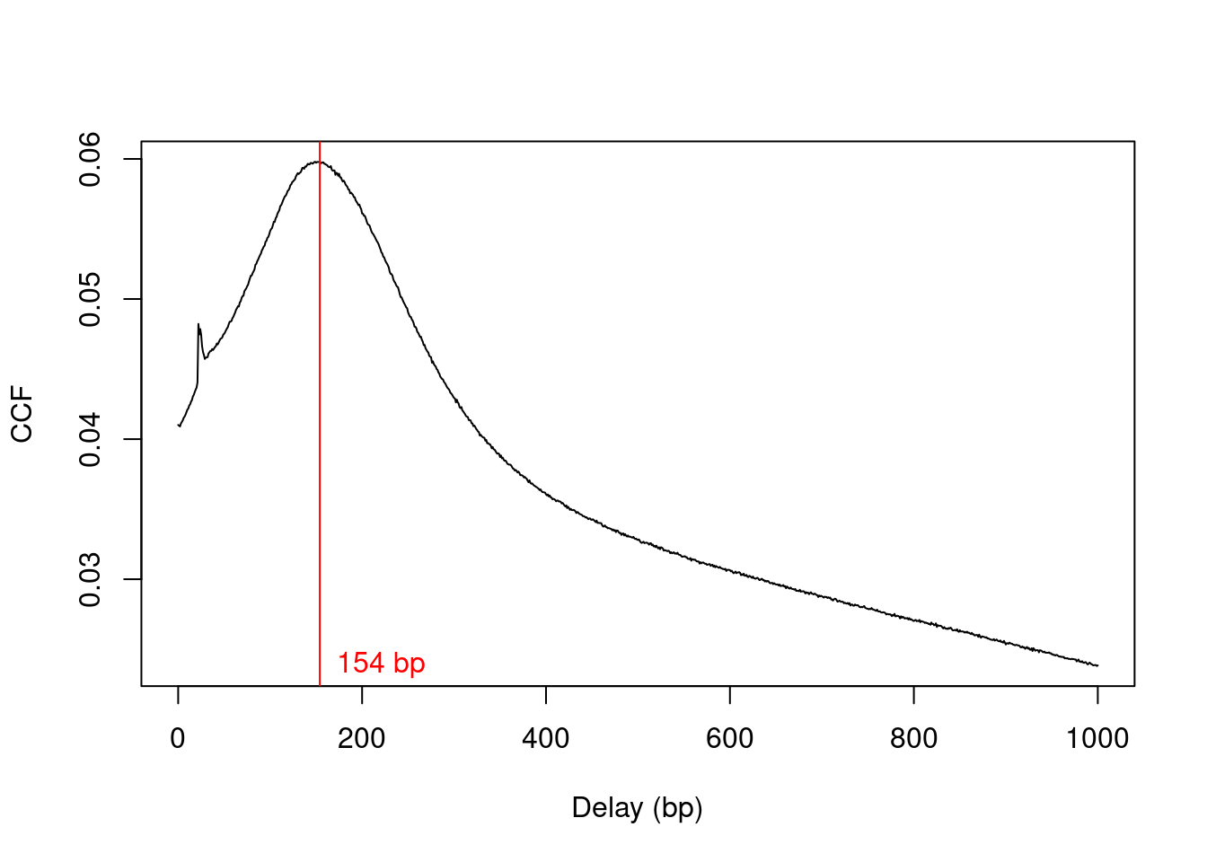
We estimate the average fragment length with cross correlation plots (Section \@ref(sec:ccf)).
Specifically, the delay at the peak in the cross correlation is used as the average length in our analysis (Figure \@ref(fig:h3k9ac-ccfplot)).
```r
x <- correlateReads(acdata$Path, param=reform(param, dedup=TRUE))
frag.len <- maximizeCcf(x)
frag.len
```
```
## [1] 154
```
```r
plot(1:length(x)-1, x, xlab="Delay (bp)", ylab="CCF", type="l")
abline(v=frag.len, col="red")
text(x=frag.len, y=min(x), paste(frag.len, "bp"), pos=4, col="red")
```
(\#fig:h3k9ac-ccfplot)Cross-correlation function (CCF) against delay distance for the H3K9ac data set. The delay with the maximum correlation is shown as the red line.
Only unmarked reads (i.e., not potential PCR duplicates) are used to calculate the cross-correlations.
However, general removal of marked reads is risky as it caps the signal in high-coverage regions of the genome.
Thus, the marking status of each read will be ignored in the rest of the analysis, i.e., no duplicates will be removed in downstream steps.
### Counting reads into windows
The `windowCounts()` function produces a `RangedSummarizedExperiment` object containing a matrix of such counts.
Each row corresponds to a window; each column represents a BAM file corresponding to a single sample^[Counting can be parallelized across files using the `BPPARAM=` argument.];
and each entry of the matrix represents the number of fragments overlapping a particular window in a particular sample.
```r
win.data <- windowCounts(acdata$Path, param=param, width=150, ext=frag.len)
win.data
```
```
## class: RangedSummarizedExperiment
## dim: 1671254 4
## metadata(6): spacing width ... param final.ext
## assays(1): counts
## rownames: NULL
## rowData names(0):
## colnames: NULL
## colData names(4): bam.files totals ext rlen
```
To analyze H3K9ac data, we use a window size of 150 bp.
This corresponds roughly to the length of the DNA in a nucleosome [@humburg2011], which is the smallest relevant unit for studying histone mark enrichment.
The spacing between windows is left as the default of 50 bp, i.e., the start positions for adjacent windows are 50 bp apart.
## Filtering windows by abundance
We remove low-abundance windows using a global filter on the background enrichment (Section \@ref(sec:global-filter)).
A window is only retained if its coverage is 3-fold higher than that of the background regions,
i.e., the abundance of the window is greater than the background abundance estimate by log~2~(3) or more.
This removes a large number of windows that are weakly or not marked and are likely to be irrelevant.
```r
bins <- windowCounts(acdata$Path, bin=TRUE, width=2000, param=param)
filter.stat <- filterWindowsGlobal(win.data, bins)
min.fc <- 3
keep <- filter.stat$filter > log2(min.fc)
summary(keep)
```
```
## Mode FALSE TRUE
## logical 982167 689087
```
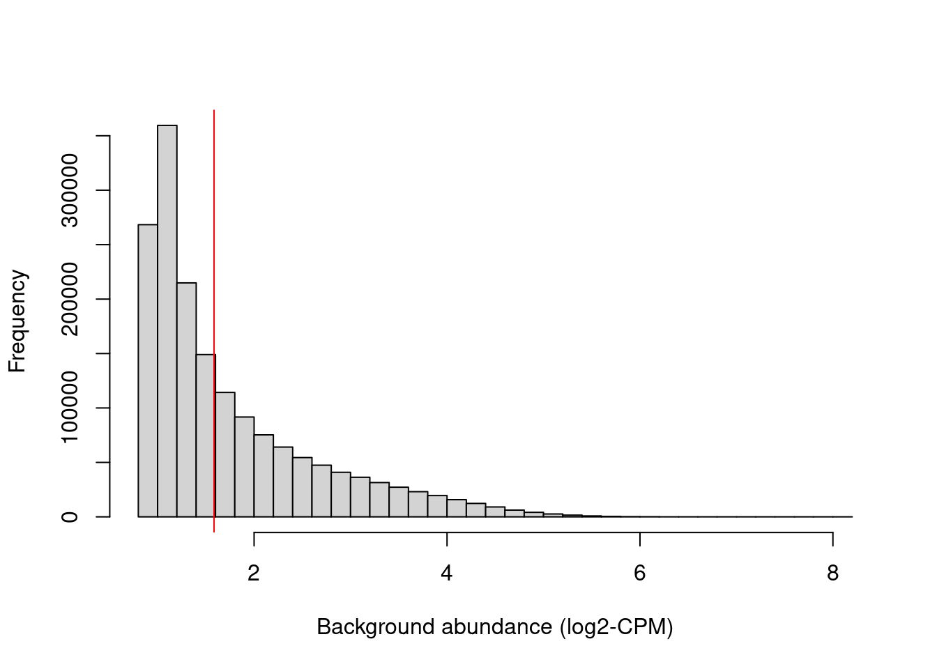
We examine the effect of the fold-change threshold in Figure \@ref(fig:h3k9ac-bghistplot).
The chosen threshold is greater than the abundances of most bins in the genome -- presumably, those that contain background regions.
This suggests that the filter will remove most windows lying within background regions.
```r
hist(filter.stat$filter, main="", breaks=50,
xlab="Background abundance (log2-CPM)")
abline(v=log2(min.fc), col="red")
```
(\#fig:h3k9ac-bghistplot)Histogram of average abundances across all 2 kbp genomic bins. The filter threshold is shown as the red line.
The filtering itself is done by simply subsetting the `RangedSummarizedExperiment` object.
```r
filtered.data <- win.data[keep,]
```
## Normalizing for trended biases
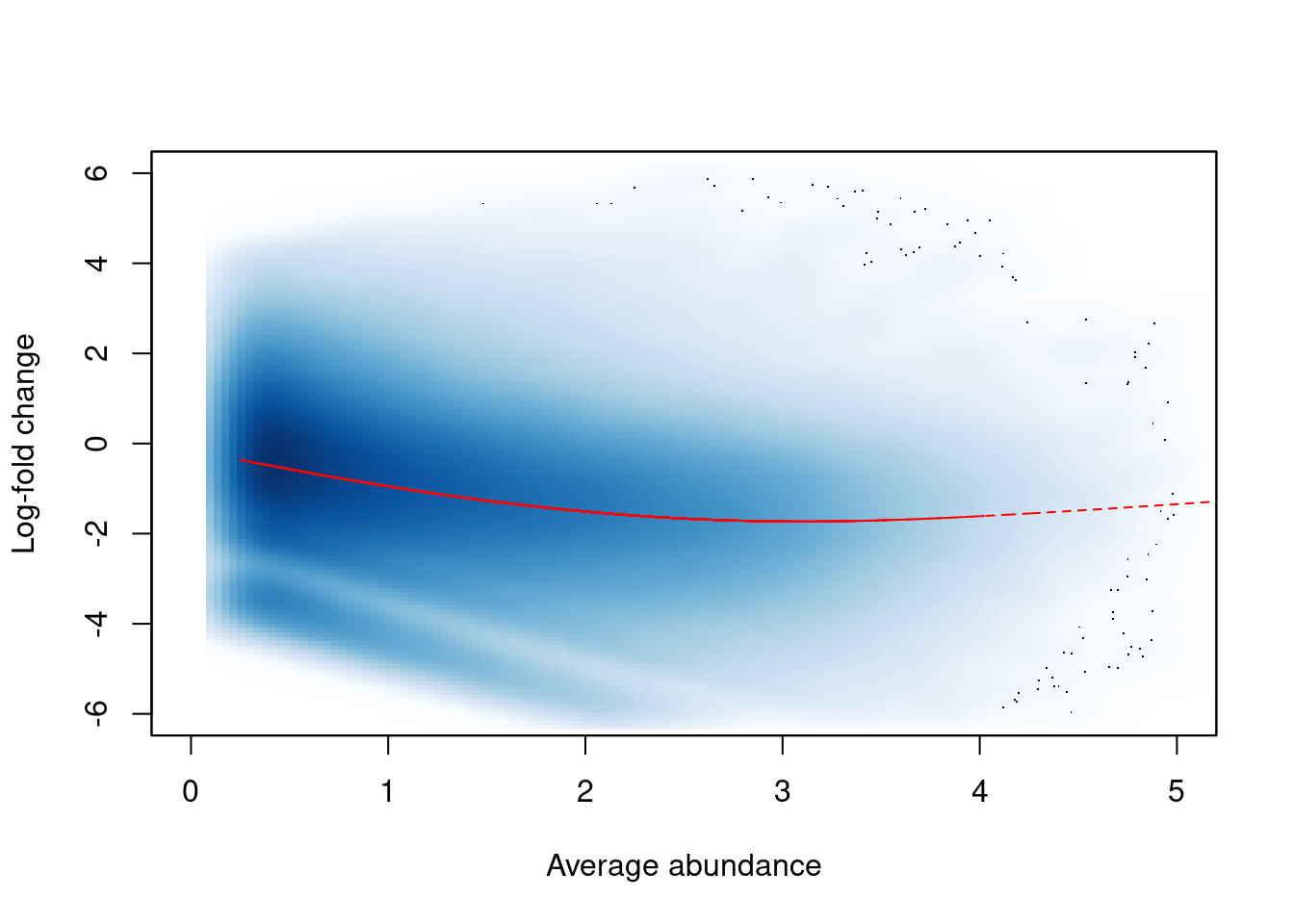
In this dataset, we observe a trended bias between samples in Figure \@ref(fig:h3k9ac-trendplot).
This refers to a systematic fold-difference in per-window coverage between samples that changes according to the average abundance of the window.
```r
win.ab <- scaledAverage(filtered.data)
adjc <- calculateCPM(filtered.data, use.offsets=FALSE)
logfc <- adjc[,4] - adjc[,1]
smoothScatter(win.ab, logfc, ylim=c(-6, 6), xlim=c(0, 5),
xlab="Average abundance", ylab="Log-fold change")
lfit <- smooth.spline(logfc~win.ab, df=5)
o <- order(win.ab)
lines(win.ab[o], fitted(lfit)[o], col="red", lty=2)
```
(\#fig:h3k9ac-trendplot)Abundance-dependent trend in the log-fold change between two H3K9ac samples (mature B over pro-B), across all windows retained after filtering. A smoothed spline fitted to the log-fold change against the average abundance is also shown in red.
To remove these biases, we use *[csaw](https://bioconductor.org/packages/3.18/csaw)* to compute a matrix of offsets for model fitting.
```r
filtered.data <- normOffsets(filtered.data)
head(assay(filtered.data, "offset"))
```
```
## [,1] [,2] [,3] [,4]
## [1,] 16.07 15.88 15.05 15.14
## [2,] 16.05 15.86 15.08 15.17
## [3,] 16.04 15.86 15.08 15.17
## [4,] 16.17 15.95 14.98 15.06
## [5,] 16.24 16.00 14.93 14.97
## [6,] 16.26 16.02 14.92 14.95
```
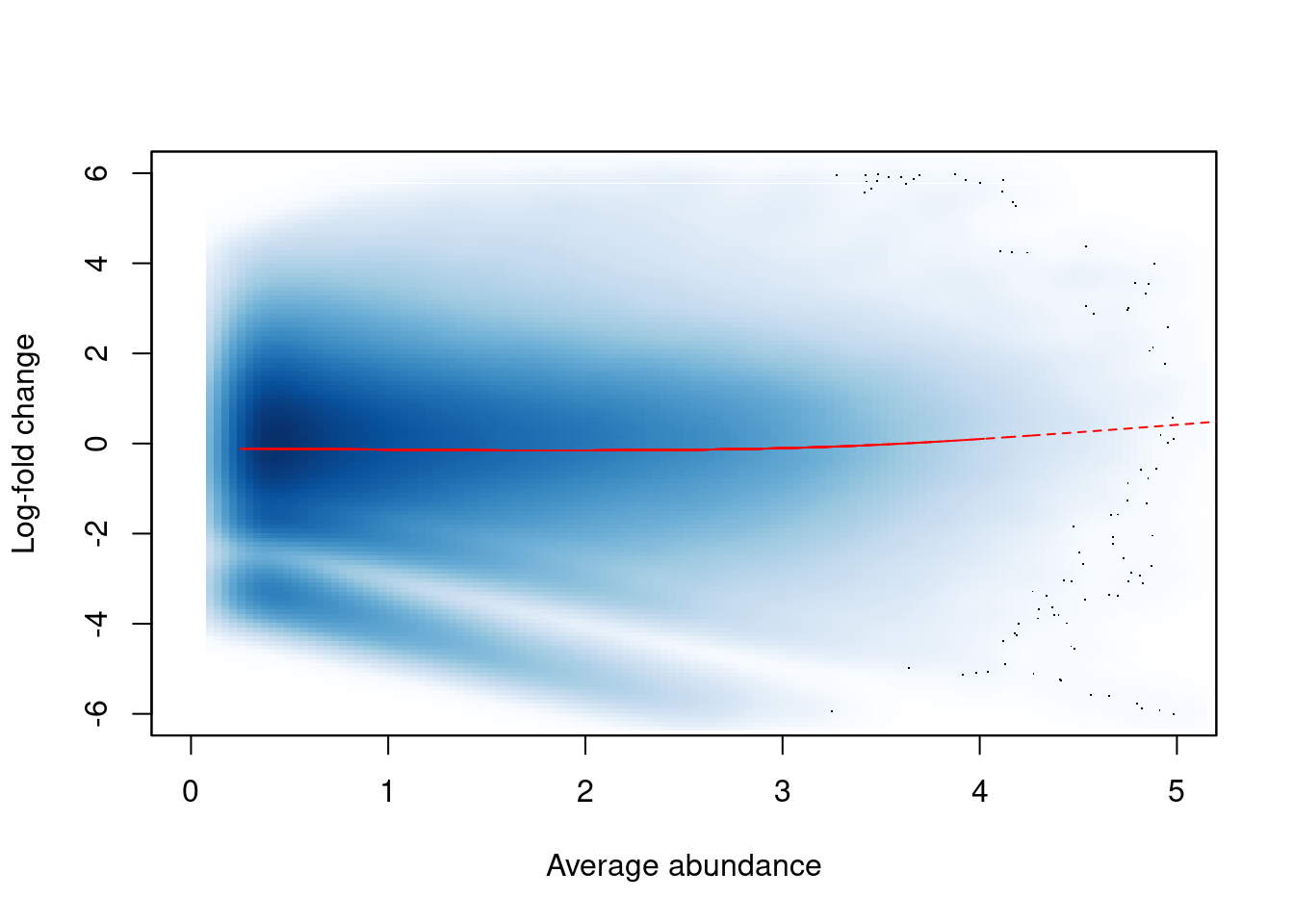
The effect of non-linear normalization is visualized with another mean-difference plot.
Once the offsets are applied to adjust the log-fold changes, the trend is eliminated from the plot (Figure \@ref(fig:h3k9ac-normplot)).
The cloud of points is also centred at a log-fold change of zero, indicating that normalization successfully removed the differences between samples.
```r
norm.adjc <- calculateCPM(filtered.data, use.offsets=TRUE)
norm.fc <- norm.adjc[,4]-norm.adjc[,1]
smoothScatter(win.ab, norm.fc, ylim=c(-6, 6), xlim=c(0, 5),
xlab="Average abundance", ylab="Log-fold change")
lfit <- smooth.spline(norm.fc~win.ab, df=5)
lines(win.ab[o], fitted(lfit)[o], col="red", lty=2)
```
(\#fig:h3k9ac-normplot)Effect of non-linear normalization on the trended bias between two H3K9ac samples. Normalized log-fold changes are shown for all windows retained after filtering. A smoothed spline fitted to the log-fold change against the average abundance is also shown in red.
The implicit assumption of non-linear methods is that most windows at each abundance are not DB.
Any systematic difference between samples is attributed to bias and is removed.
The assumption of a non-DB majority is reasonable for this data set, given that the cell types being compared are quite closely related.
## Statistical modelling
### Estimating the NB dispersion
First, we set up our design matrix.
This involves a fairly straightforward one-way layout with the groups representing our two cell types.
```r
celltype <- acdata$Description
celltype[grep("pro", celltype)] <- "proB"
celltype[grep("mature", celltype)] <- "matureB"
celltype <- factor(celltype)
design <- model.matrix(~0+celltype)
colnames(design) <- levels(celltype)
design
```
```
## matureB proB
## 1 0 1
## 2 0 1
## 3 1 0
## 4 1 0
## attr(,"assign")
## [1] 1 1
## attr(,"contrasts")
## attr(,"contrasts")$celltype
## [1] "contr.treatment"
```
We coerce the `RangedSummarizedExperiment` object into a `DGEList` object (plus offsets) for use in *[edgeR](https://bioconductor.org/packages/3.18/edgeR)*.
We then estimate the NB dispersion to capture the mean-variance relationship.
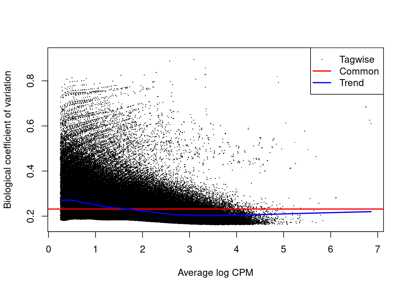
The NB dispersion estimates are shown in Figure \@ref(fig:h3k9ac-bcvplot) as their square roots, i.e., the biological coefficients of variation.
Data sets with common BCVs ranging from 10 to 20% are considered to have low variability for ChIP-seq experiments.
```r
library(edgeR)
y <- asDGEList(filtered.data)
str(y)
```
```
## Formal class 'DGEList' [package "edgeR"] with 1 slot
## ..@ .Data:List of 3
## .. ..$ : int [1:689087, 1:4] 6 6 7 12 15 17 24 22 25 24 ...
## .. .. ..- attr(*, "dimnames")=List of 2
## .. .. .. ..$ : chr [1:689087] "1" "2" "3" "4" ...
## .. .. .. ..$ : chr [1:4] "Sample1" "Sample2" "Sample3" "Sample4"
## .. ..$ :'data.frame': 4 obs. of 3 variables:
## .. .. ..$ group : Factor w/ 1 level "1": 1 1 1 1
## .. .. ..$ lib.size : int [1:4] 8392971 7269175 3792141 4241789
## .. .. ..$ norm.factors: num [1:4] 1 1 1 1
## .. ..$ : num [1:689087, 1:4] 16.1 16 16 16.2 16.2 ...
## ..$ names: chr [1:3] "counts" "samples" "offset"
```
```r
y <- estimateDisp(y, design)
summary(y$trended.dispersion)
```
```
## Min. 1st Qu. Median Mean 3rd Qu. Max.
## 0.0410 0.0525 0.0617 0.0607 0.0721 0.0740
```
```r
plotBCV(y)
```
(\#fig:h3k9ac-bcvplot)Abundance-dependent trend in the BCV for each window, represented by the blue line. Common (red) and tagwise estimates (black) are also shown.
### Estimating the QL dispersion
We use quasi-likelihood methods to model window-specific variability, i.e., variance in the variance across windows.
However, with limited replicates, there is not enough information for each window to stably estimate the QL dispersion.
This is overcome by sharing information between windows with empirical Bayes (EB) shrinkage.
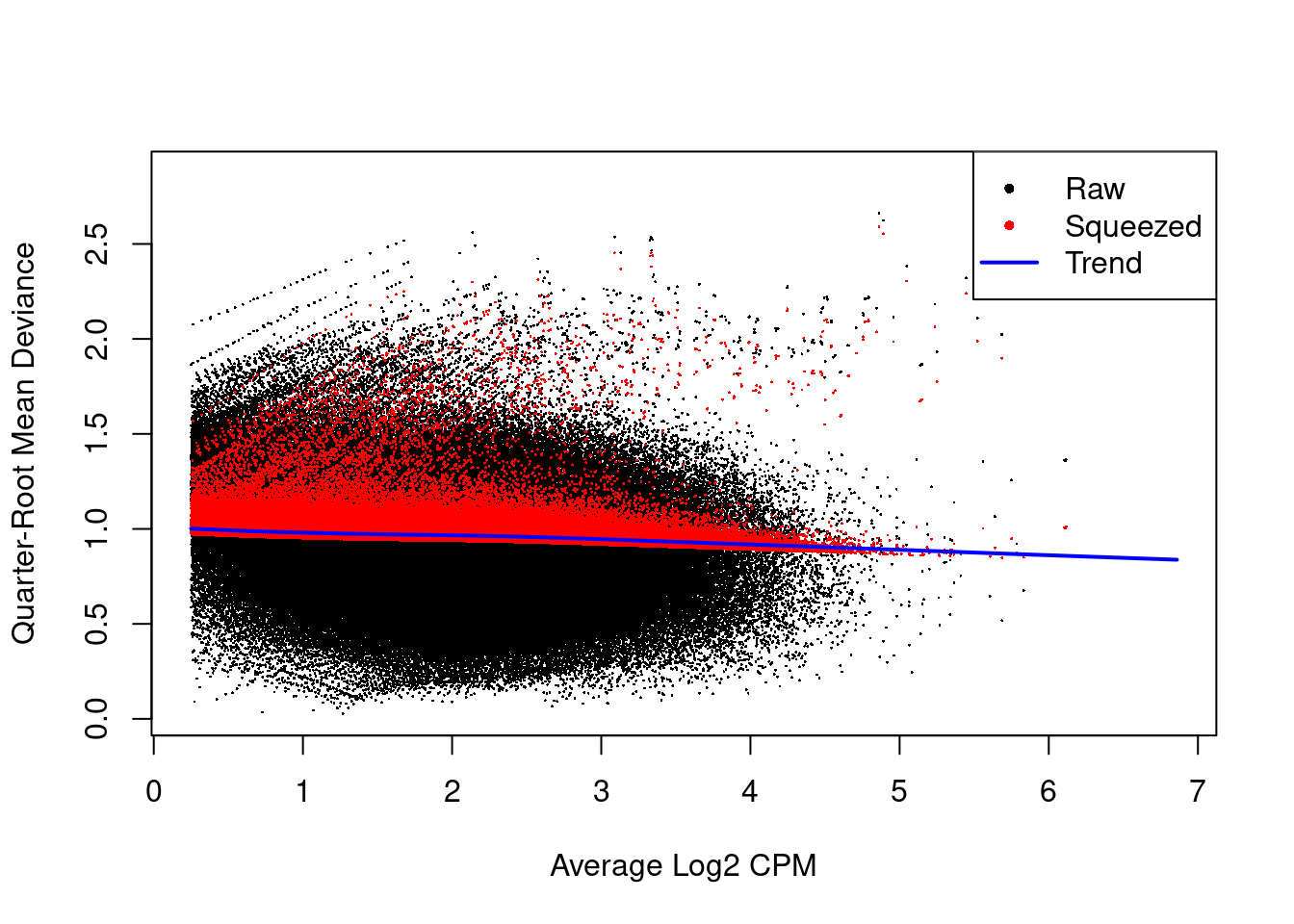
The instability of the QL dispersion estimates is reduced by squeezing the estimates towards an abundance-dependent trend (Figure \@ref(fig:h3k9ac-qlplot)).
```r
fit <- glmQLFit(y, design, robust=TRUE)
plotQLDisp(fit)
```
(\#fig:h3k9ac-qlplot)Effect of EB shrinkage on the raw QL dispersion estimate for each window (black) towards the abundance-dependent trend (blue) to obtain squeezed estimates (red).
The extent of shrinkage is determined by the prior degrees of freedom (d.f.).
Large prior d.f. indicates that the dispersions were similar across windows, such that stronger shrinkage to the trend could be performed to increase stability and power.
```r
summary(fit$df.prior)
```
```
## Min. 1st Qu. Median Mean 3rd Qu. Max.
## 0.224 15.495 15.495 15.254 15.495 15.495
```
Also note the use of `robust=TRUE` in the `glmQLFit()` call, which reduces the sensitivity of the EB procedures to outlier variances.
This is particularly noticeable in Figure \@ref(fig:h3k9ac-qlplot) with highly variable windows that (correctly) do not get squeezed towards the trend.
### Examining the data with MDS plots
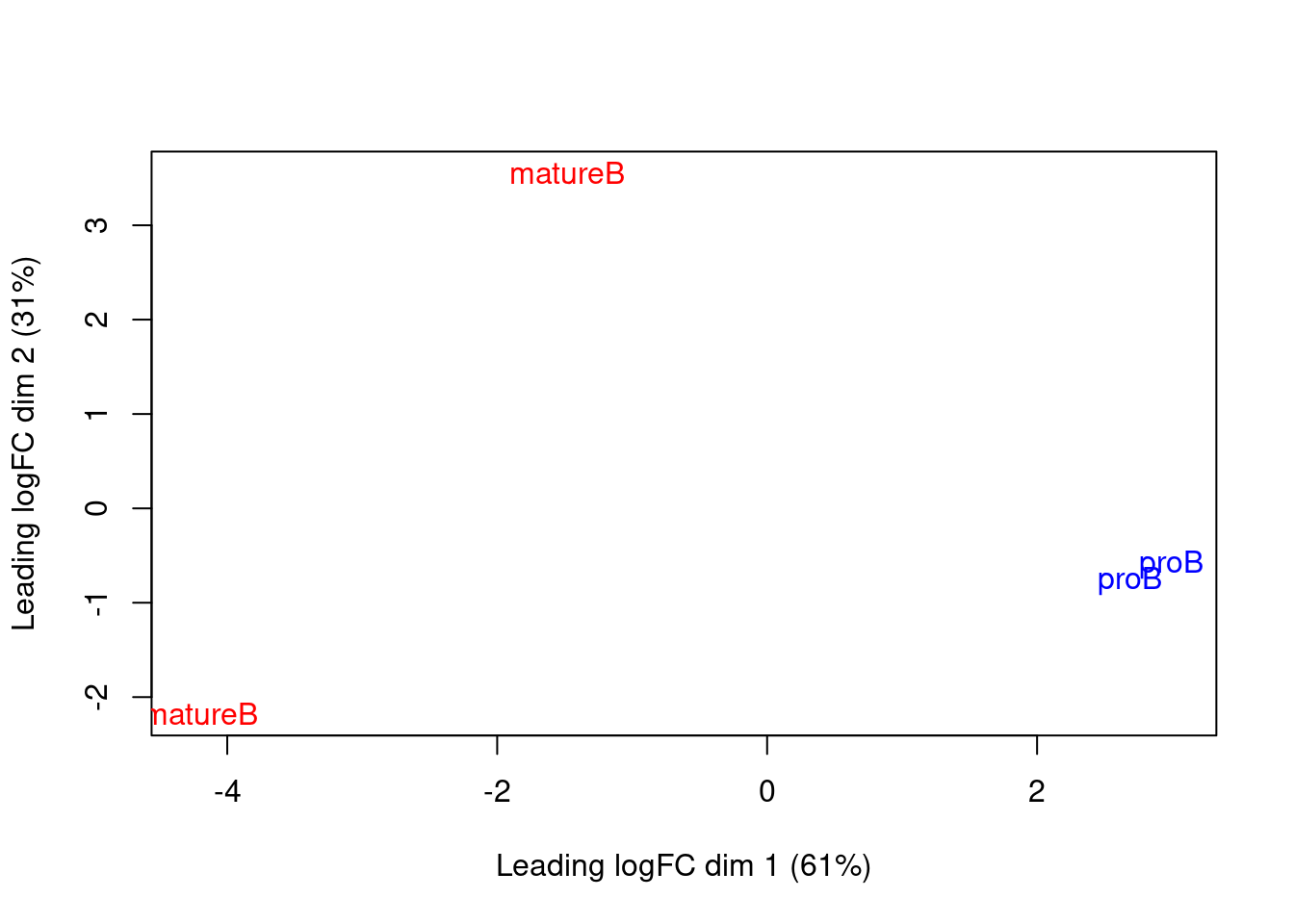
We use MDS plots to examine the similarities between samples.
Ideally, replicates should cluster together while samples from different conditions should be separate.
While the mature B replicates are less tightly grouped, samples still separate by cell type in Figure \@ref(fig:h3k9ac-mdsplot).
This suggests that our downstream analysis will be able to detect significant differences in enrichment between cell types.
```r
plotMDS(norm.adjc, labels=celltype,
col=c("red", "blue")[as.integer(celltype)])
```
(\#fig:h3k9ac-mdsplot)MDS plot with two dimensions for all samples in the H3K9ac data set. Samples are labelled and coloured according to the cell type.
## Testing for DB
Each window is tested for significant differences between cell types using the QL F-test.
For this analysis, the comparison is parametrized such that the reported log-fold change for each window represents that of the coverage in pro-B cells over their mature B counterparts.
```r
contrast <- makeContrasts(proB-matureB, levels=design)
res <- glmQLFTest(fit, contrast=contrast)
head(res$table)
```
```
## logFC logCPM F PValue
## 1 1.3658 0.3097 2.306 0.14678
## 2 1.3564 0.2624 2.305 0.14685
## 3 2.0015 0.2503 3.940 0.06305
## 4 2.0780 0.5033 5.576 0.03003
## 5 0.8842 0.8051 1.652 0.21545
## 6 0.9678 0.8949 2.055 0.16936
```
We then control the region-level FDR by aggregating windows into regions and combining the $p$-values.
Here, adjacent windows less than 100 bp apart are aggregated into clusters.
```r
merged <- mergeResults(filtered.data, res$table, tol=100,
merge.args=list(max.width=5000))
merged$regions
```
```
## GRanges object with 41616 ranges and 0 metadata columns:
## seqnames ranges strand
##
## [1] chr1 4775451-4775750 *
## [2] chr1 4785001-4786300 *
## [3] chr1 4807251-4807750 *
## [4] chr1 4808001-4808600 *
## [5] chr1 4857051-4858950 *
## ... ... ... ...
## [41612] chrY 73038001-73038400 *
## [41613] chrY 75445801-75446200 *
## [41614] chrY 88935951-88936350 *
## [41615] chrY 90554201-90554400 *
## [41616] chrY 90812801-90813100 *
## -------
## seqinfo: 21 sequences from an unspecified genome
```
A combined $p$-value is computed for each cluster using the method of @simes1986, based on the $p$-values of the constituent windows.
This represents the evidence against the global null hypothesis for each cluster, i.e., that no DB exists in any of its windows.
Rejection of this global null indicates that the cluster (and the region that it represents) contains DB.
Applying the BH method to the combined $p$-values allows the region-level FDR to be controlled.
```r
tabcom <- merged$combined
tabcom
```
```
## DataFrame with 41616 rows and 8 columns
## num.tests num.up.logFC num.down.logFC PValue FDR direction
##
## 1 3 0 0 0.1468526 0.2464281 up
## 2 24 0 0 0.0882967 0.1687355 up
## 3 8 0 0 0.5264245 0.6480413 mixed
## 4 10 0 0 0.7296509 0.8298757 mixed
## 5 36 5 0 0.0208882 0.0605414 up
## ... ... ... ... ... ... ...
## 41612 6 0 6 0.00587505 0.0265930 down
## 41613 6 0 6 0.03868017 0.0930955 down
## 41614 6 0 6 0.02082155 0.0604134 down
## 41615 2 0 2 0.03344646 0.0836785 down
## 41616 4 0 4 0.00147494 0.0114325 down
## rep.test rep.logFC
##
## 1 2 1.356426
## 2 15 6.454882
## 3 34 0.433617
## 4 40 -0.272420
## 5 63 6.353706
## ... ... ...
## 41612 689066 -6.96911
## 41613 689075 -5.73312
## 41614 689081 -5.84635
## 41615 689083 -5.00404
## 41616 689087 -3.96416
```
We determine the total number of DB regions at a FDR of 5%
by applying the Benjamini-Hochberg method on the combined $p$-values.
```r
is.sig <- tabcom$FDR <= 0.05
summary(is.sig)
```
```
## Mode FALSE TRUE
## logical 28515 13101
```
Determining the direction of DB is more complicated, as clusters may contain windows that are changing in opposite directions.
One approach is to use the direction of DB from the windows that contribute most to the combined $p$-value,
as reported in the `direction` field for each cluster.
```r
table(tabcom$direction[is.sig])
```
```
##
## down mixed up
## 8580 154 4367
```
Another approach is to use the log-fold change of the most significant window as a proxy for the log-fold change of the cluster.
```r
tabbest <- merged$best
tabbest
```
```
## DataFrame with 41616 rows and 8 columns
## num.tests num.up.logFC num.down.logFC PValue FDR direction
##
## 1 3 0 0 0.1891477 0.335560 up
## 2 24 0 0 0.0882967 0.190583 up
## 3 8 0 0 1.0000000 1.000000 up
## 4 10 0 0 1.0000000 1.000000 down
## 5 36 2 0 0.0464346 0.121536 up
## ... ... ... ... ... ... ...
## 41612 6 0 3 0.01762514 0.0634640 down
## 41613 6 0 0 0.19568010 0.3445628 down
## 41614 6 0 0 0.06141175 0.1463585 down
## 41615 2 0 0 0.06689293 0.1549923 down
## 41616 4 0 4 0.00421597 0.0261244 down
## rep.test rep.logFC
##
## 1 3 2.001538
## 2 15 6.454882
## 3 35 1.178400
## 4 43 -0.908825
## 5 60 6.572738
## ... ... ...
## 41612 689064 -6.96911
## 41613 689070 -5.44350
## 41614 689076 -6.68322
## 41615 689082 -5.00404
## 41616 689086 -4.08131
```
In the table above, the `rep.test` column is the index of the window that is the most significant in each cluster,
while the `rep.logFC` field is the log-fold change of that window.
We could also use this to obtain a summary of the direction of DB across all clusters.
```r
is.sig.pos <- (tabbest$rep.logFC > 0)[is.sig]
summary(is.sig.pos)
```
```
## Mode FALSE TRUE
## logical 8664 4437
```
The final approach is generally satisfactory, though it will not capture multiple changes in opposite directions^[Try `mixedClusters()` to formally detect clusters that contain significant changes in both directions.].
It also tends to overstate the magnitude of the log-fold change in each cluster.
## Interpreting the DB results
### Adding gene-centric annotation
For convenience, we store all statistics in the metadata of a `GRanges` object.
We also store the midpoint and log-fold change of the most significant window in each cluster.
```r
out.ranges <- merged$regions
mcols(out.ranges) <- DataFrame(tabcom,
best.pos=mid(ranges(rowRanges(filtered.data[tabbest$rep.test]))),
best.logFC=tabbest$rep.logFC)
```
We can then use the built-in annotation function in *[csaw](https://bioconductor.org/packages/3.18/csaw)* to report genic features overlapping to each region (Section \@ref(sec:detail-ranges)).
Annotated features that flank the region of interest are also reported.
```r
library(org.Mm.eg.db)
library(TxDb.Mmusculus.UCSC.mm10.knownGene)
anno <- detailRanges(out.ranges, orgdb=org.Mm.eg.db,
txdb=TxDb.Mmusculus.UCSC.mm10.knownGene)
head(anno$overlap)
```
```
## [1] "Mrpl15:-:E" "Mrpl15:-:PE" "Lypla1:+:P"
## [4] "Lypla1:+:PE" "Lypla1:+:I,Tcea1:+:PE" "Rgs20:-:I"
```
```r
head(anno$left)
```
```
## [1] "Mrpl15:-:935" "Mrpl15:-:896" "" "Lypla1:+:19" ""
## [6] ""
```
```r
head(anno$right)
```
```
## [1] "Mrpl15:-:627" "" "Lypla1:+:38" "" ""
## [6] ""
```
The annotation for each region is stored in the metadata of the `GRanges` object.
The compact string form is useful for human interpretation, as it allows rapid examination of all genic features neighbouring each region.
```r
meta <- mcols(out.ranges)
mcols(out.ranges) <- data.frame(meta, anno)
```
### Using the *[ChIPpeakAnno](https://bioconductor.org/packages/3.18/ChIPpeakAnno)* package
As its name suggests, the *[ChIPpeakAnno](https://bioconductor.org/packages/3.18/ChIPpeakAnno)* package is designed to annotate peaks from ChIP-seq experiments [@zhu2010chippeakanno].
A `GRanges` object containing all regions of interest is supplied to the relevant function after removing all previous metadata fields to reduce clutter.
The gene closest to each region is then reported.
Gene coordinates are taken from the NCBI mouse 38 annotation, which is roughly equivalent to the annotation in the mm10 genome build.
```r
library(ChIPpeakAnno)
data(TSS.mouse.GRCm38)
minimal <- out.ranges
elementMetadata(minimal) <- NULL
anno.regions <- annotatePeakInBatch(minimal, AnnotationData=TSS.mouse.GRCm38)
colnames(elementMetadata(anno.regions))
```
```
## [1] "peak" "feature"
## [3] "start_position" "end_position"
## [5] "feature_strand" "insideFeature"
## [7] "distancetoFeature" "shortestDistance"
## [9] "fromOverlappingOrNearest"
```
Alternatively, identification of all overlapping features within, say, 5 kbp can be achieved by setting `maxgap=5000` and `output="overlapping"` in `annotatePeakInBatch`.
This will report each overlapping feature in a separate entry of the returned `GRanges` object, i.e., each input region may have multiple output values.
In contrast, `detailRanges()` will report all overlapping features for a region as a single string, i.e., each input region has one output value.
Which is preferable depends on the purpose of the annotation -- the `detailRanges()` output is more convenient for direct annotation of a DB list, while the `annotatePeakInBatch()` output contains more information and is more convenient for further manipulation.
### Reporting gene-based results
Another approach to annotation is to flip the problem around such that DB statistics are reported directly for features of interest like genes.
This is more convenient when the DB analysis needs to be integrated with, e.g., differential expression analyses of matched RNA-seq data.
In the code below, promoter coordinates and gene symbols are obtained from various annotation objects.
```r
prom <- suppressWarnings(promoters(TxDb.Mmusculus.UCSC.mm10.knownGene,
upstream=3000, downstream=1000, columns=c("tx_name", "gene_id")))
entrez.ids <- sapply(prom$gene_id, FUN=function(x) x[1]) # Using the first Entrez ID.
gene.name <- select(org.Mm.eg.db, keys=entrez.ids, keytype="ENTREZID", column="SYMBOL")
prom$gene_name <- gene.name$SYMBOL[match(entrez.ids, gene.name$ENTREZID)]
head(prom)
```
```
## GRanges object with 6 ranges and 3 metadata columns:
## seqnames ranges strand | tx_name
## |
## ENSMUST00000193812.1 chr1 3070253-3074252 + | ENSMUST00000193812.1
## ENSMUST00000082908.1 chr1 3099016-3103015 + | ENSMUST00000082908.1
## ENSMUST00000192857.1 chr1 3249757-3253756 + | ENSMUST00000192857.1
## ENSMUST00000161581.1 chr1 3463587-3467586 + | ENSMUST00000161581.1
## ENSMUST00000192183.1 chr1 3528795-3532794 + | ENSMUST00000192183.1
## ENSMUST00000193244.1 chr1 3677155-3681154 + | ENSMUST00000193244.1
## gene_id gene_name
##
## ENSMUST00000193812.1
## ENSMUST00000082908.1
## ENSMUST00000192857.1
## ENSMUST00000161581.1
## ENSMUST00000192183.1
## ENSMUST00000193244.1
## -------
## seqinfo: 66 sequences (1 circular) from mm10 genome
```
All windows overlapping each promoter are defined as a cluster.
We compute DB statistics are computed for each cluster/promoter using Simes' method,
which directly yields DB results for the annotated features.
Promoters with no overlapping windows are assigned `NA` values for the various fields and are filtered out below for demonstration purposes.
```r
olap.out <- overlapResults(filtered.data, regions=prom, res$table)
olap.out
```
```
## DataFrame with 142446 rows and 3 columns
## regions combined best
##
## 1 chr1:3070253-3074252:+ NA:NA:NA:... NA:NA:NA:...
## 2 chr1:3099016-3103015:+ NA:NA:NA:... NA:NA:NA:...
## 3 chr1:3249757-3253756:+ NA:NA:NA:... NA:NA:NA:...
## 4 chr1:3463587-3467586:+ NA:NA:NA:... NA:NA:NA:...
## 5 chr1:3528795-3532794:+ NA:NA:NA:... NA:NA:NA:...
## ... ... ... ...
## 142442 chrUn_GL456381:15722-19721:- NA:NA:NA:... NA:NA:NA:...
## 142443 chrUn_GL456385:28243-32242:+ NA:NA:NA:... NA:NA:NA:...
## 142444 chrUn_GL456385:29719-33718:+ NA:NA:NA:... NA:NA:NA:...
## 142445 chrUn_JH584304:58668-62667:- NA:NA:NA:... NA:NA:NA:...
## 142446 chrUn_JH584304:58691-62690:- NA:NA:NA:... NA:NA:NA:...
```
```r
simple <- DataFrame(ID=prom$tx_name, Gene=prom$gene_name, olap.out$combined)
simple[!is.na(simple$PValue),]
```
```
## DataFrame with 57380 rows and 10 columns
## ID Gene num.tests num.up.logFC num.down.logFC
##
## 1 ENSMUST00000134384.7 Lypla1 18 0 0
## 2 ENSMUST00000027036.10 Lypla1 18 0 0
## 3 ENSMUST00000150971.7 Lypla1 18 0 0
## 4 ENSMUST00000155020.1 Lypla1 18 0 0
## 5 ENSMUST00000119612.8 Lypla1 18 0 0
## ... ... ... ... ... ...
## 57376 ENSMUST00000150715.1 Uty 18 0 11
## 57377 ENSMUST00000154527.1 Uty 18 0 11
## 57378 ENSMUST00000091190.11 Ddx3y 17 0 17
## 57379 ENSMUST00000188484.1 Ddx3y 17 0 17
## 57380 ENSMUST00000187962.1 NA 3 0 3
## PValue FDR direction rep.test rep.logFC
##
## 1 0.700465 0.739135 mixed 40 -0.27242
## 2 0.700465 0.739135 mixed 40 -0.27242
## 3 0.700465 0.739135 mixed 40 -0.27242
## 4 0.700465 0.739135 mixed 40 -0.27242
## 5 0.700465 0.739135 mixed 40 -0.27242
## ... ... ... ... ... ...
## 57376 6.45130e-06 0.000324147 down 689012 -3.36536
## 57377 6.45130e-06 0.000324147 down 689012 -3.36536
## 57378 6.82321e-05 0.001421855 down 689019 -2.78424
## 57379 6.82321e-05 0.001421855 down 689019 -2.78424
## 57380 2.93752e-03 0.013802417 down 689066 -6.96911
```
Note that this strategy is distinct from counting reads across promoters.
Using promoter-level counts would not provide enough spatial resolution to detect sharp binding events that only occur in a subinterval of the promoter.
In particular, detection may be compromised by non-specific background or the presence of multiple opposing DB events in the same promoter.
Combining window-level statistics is preferable as resolution is maintained for optimal performance.
## Visualizing DB results
### Overview
We again use the *[Gviz](https://bioconductor.org/packages/3.18/Gviz)* package to visualize read coverage across the data set at regions of interest [@hahne2016visualizing].
Coverage in each BAM file will be represented by a single track.
Several additional tracks will also be included in each plot.
One is the genome axis track, to display the genomic coordinates across the plotted region.
The other is the annotation track containing gene models, with gene IDs replaced by symbols (where possible) for easier reading.
```r
library(Gviz)
gax <- GenomeAxisTrack(col="black", fontsize=15, size=2)
greg <- GeneRegionTrack(TxDb.Mmusculus.UCSC.mm10.knownGene, showId=TRUE,
geneSymbol=TRUE, name="", background.title="transparent")
symbols <- unlist(mapIds(org.Mm.eg.db, gene(greg), "SYMBOL",
"ENTREZID", multiVals = "first"))
symbol(greg) <- symbols[gene(greg)]
```
We will also sort the DB regions by p-value for easier identification of regions of interest.
```r
o <- order(out.ranges$PValue)
sorted.ranges <- out.ranges[o]
sorted.ranges
```
```
## GRanges object with 41616 ranges and 13 metadata columns:
## seqnames ranges strand | num.tests num.up.logFC
## |
## [1] chr17 34285101-34290050 * | 97 0
## [2] chr9 109050201-109053150 * | 57 0
## [3] chr17 34261151-34265850 * | 92 5
## [4] chr17 34306001-34308650 * | 51 0
## [5] chr18 60802751-60805750 * | 55 0
## ... ... ... ... . ... ...
## [41612] chr18 23751901-23753200 * | 22 0
## [41613] chr12 83922051-83922650 * | 10 0
## [41614] chr15 99395101-99395650 * | 8 0
## [41615] chr3 67504201-67504500 * | 4 0
## [41616] chr4 43043401-43043700 * | 4 0
## num.down.logFC PValue FDR direction rep.test
##
## [1] 97 4.04798e-11 1.22570e-06 down 291020
## [2] 57 7.13784e-11 1.22570e-06 down 671262
## [3] 74 8.83575e-11 1.22570e-06 down 290891
## [4] 51 1.23282e-10 1.28263e-06 down 291358
## [5] 55 2.06286e-10 1.54430e-06 down 321713
## ... ... ... ... ... ...
## [41612] 0 0.999833 0.999908 mixed 313278
## [41613] 0 0.999885 0.999908 mixed 153754
## [41614] 0 0.999908 0.999908 mixed 247763
## [41615] 0 0.999908 0.999908 up 416884
## [41616] 0 0.999908 0.999908 mixed 443668
## rep.logFC best.pos best.logFC overlap
##
## [1] -6.97365 34287575 -7.18686 H2-Aa:-:PE
## [2] -5.84054 109051575 -6.19603 Shisa5:+:PE
## [3] -7.87978 34262025 -7.70115 H2-Ab1:+:PE
## [4] -6.86030 34306075 -5.80798 H2-Eb1:+:PE
## [5] -5.13082 60804525 -5.98346 Cd74:+:PE
## ... ... ... ... ...
## [41612] -0.000502650 23752525 -0.777050 Gm15972:-:PE,Mapre2:..
## [41613] 0.000405487 83922125 0.880875 Numb:-:P
## [41614] 0.000119628 99395425 -0.411300 Tmbim6:+:I
## [41615] 0.000119628 67504275 0.491618 Rarres1:-:I
## [41616] 0.000119628 43043575 0.174254 Atosb:-:I
## left right
##
## [1] H2-Aa:-:565
## [2] Gm53191:-:4783,Trex1..
## [3] H2-Ab1:+:3314 H2-Ab1:+:1252
## [4] H2-Eb1:+:925
## [5] Cd74:+:2158
## ... ... ...
## [41612] Gm15972:-:78 Mapre2:+:525
## [41613] Numb:-:117
## [41614] Tmbim6:+:1371 Tmbim6:+:4007
## [41615]
## [41616] Atosb:-:3106 Atosb:-:1948
## -------
## seqinfo: 21 sequences from an unspecified genome
```
### Simple DB across a broad region
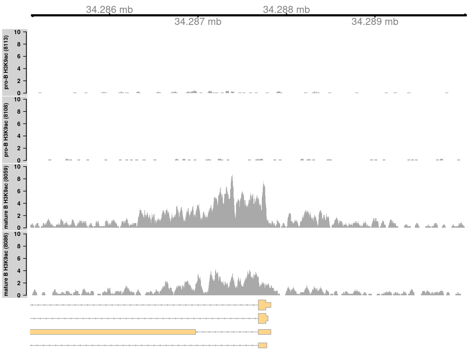
We start by visualizing one of the top-ranking DB regions.
This represents a simple DB event where the entire region changes in one direction (Figure \@ref(fig:simplebroadplot)).
Specifically, it represents an increase in H3K9ac marking at the *H2-Aa* locus in mature B cells.
This is consistent with the expected biology -- H3K9ac is a mark of active gene expression and MHCII components are upregulated in mature B cells [@hoffman2002changes].
```r
cur.region <- sorted.ranges[1]
cur.region
```
```
## GRanges object with 1 range and 13 metadata columns:
## seqnames ranges strand | num.tests num.up.logFC num.down.logFC
## |
## [1] chr17 34285101-34290050 * | 97 0 97
## PValue FDR direction rep.test rep.logFC best.pos
##
## [1] 4.04798e-11 1.2257e-06 down 291020 -6.97365 34287575
## best.logFC overlap left right
##
## [1] -7.18686 H2-Aa:-:PE H2-Aa:-:565
## -------
## seqinfo: 21 sequences from an unspecified genome
```
One track is plotted for each sample, in addition to the coordinate and annotation tracks.
Coverage is plotted in terms of sequencing depth-per-million at each base.
This corrects for differences in library sizes between tracks.
```r
collected <- list()
lib.sizes <- filtered.data$totals/1e6
for (i in seq_along(acdata$Path)) {
reads <- extractReads(bam.file=acdata$Path[[i]], cur.region, param=param)
cov <- as(coverage(reads)/lib.sizes[i], "GRanges")
collected[[i]] <- DataTrack(cov, type="histogram", lwd=0, ylim=c(0,10),
name=acdata$Description[i], col.axis="black", col.title="black",
fill="darkgray", col.histogram=NA)
}
plotTracks(c(gax, collected, greg), chromosome=as.character(seqnames(cur.region)),
from=start(cur.region), to=end(cur.region))
```
(\#fig:simplebroadplot)Coverage tracks for a simple DB event between pro-B and mature B cells, across a broad region in the H3K9ac data set. Read coverage for each sample is shown as a per-million value at each base.
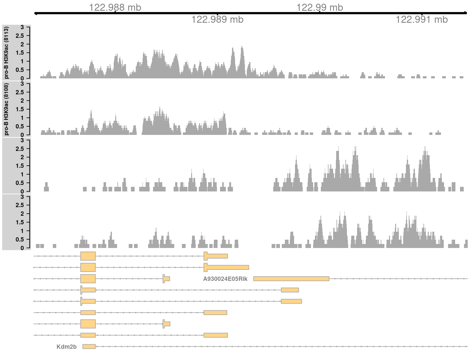
## Complex DB across a broad region
Complex DB refers to situations where multiple DB events are occurring within the same enriched region.
These are identified as those clusters that contain windows changing in both directions^[Technically, we should use `mixedClusters()` for rigorous identification of regions with significant changes in both directions. However, for simplicity, we'll just use a more _ad hoc_ approach here.].
Here, one of the top-ranking complex clusters is selected for visualization.
```r
complex <- sorted.ranges$num.up.logFC > 0 & sorted.ranges$num.down.logFC > 0
cur.region <- sorted.ranges[complex][2]
cur.region
```
```
## GRanges object with 1 range and 13 metadata columns:
## seqnames ranges strand | num.tests num.up.logFC
## |
## [1] chr5 122987201-122991450 * | 83 5
## num.down.logFC PValue FDR direction rep.test rep.logFC
##
## [1] 37 1.30976e-08 1.33826e-05 down 508657 -5.8272
## best.pos best.logFC overlap left
##
## [1] 122990925 -5.48535 A930024E05Rik:+:PE,K.. Kdm2b:-:2230
## right
##
## [1] A930024E05Rik:+:2913
## -------
## seqinfo: 21 sequences from an unspecified genome
```
This region contains a bidirectional promoter where different genes are marked in the different cell types (Figure \@ref(fig:complexplot)).
Upon differentiation to mature B cells, loss of marking in one part of the region is balanced by a gain in marking in another part of the region.
This represents a complex DB event that would not be detected if reads were counted across the entire region.
```r
collected <- list()
for (i in seq_along(acdata$Path)) {
reads <- extractReads(bam.file=acdata$Path[[i]], cur.region, param=param)
cov <- as(coverage(reads)/lib.sizes[i], "GRanges")
collected[[i]] <- DataTrack(cov, type="histogram", lwd=0, ylim=c(0,3),
name=acdata$Description[i], col.axis="black", col.title="black",
fill="darkgray", col.histogram=NA)
}
plotTracks(c(gax, collected, greg), chromosome=as.character(seqnames(cur.region)),
from=start(cur.region), to=end(cur.region))
```
(\#fig:complexplot)Coverage tracks for a complex DB event in the H3K9ac data set, shown as per-million values.
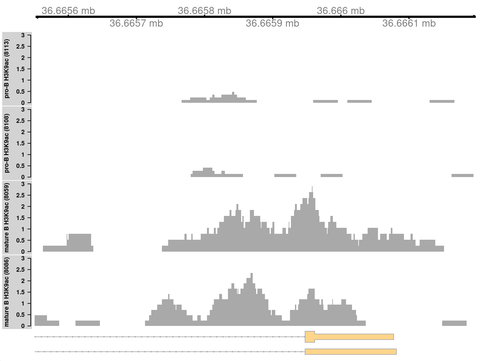
### Simple DB across a small region
Both of the examples above involve differential marking within broad regions spanning several kilobases.
This is consistent with changes in the marking profile across a large number of nucleosomes.
However, H3K9ac marking can also be concentrated into small regions, involving only a few nucleosomes.
*[csaw](https://bioconductor.org/packages/3.18/csaw)* is equally capable of detecting sharp DB within these small regions.
This is demonstrated by examining those clusters that contain a smaller number of windows.
```r
sharp <- sorted.ranges$num.tests < 20
cur.region <- sorted.ranges[sharp][1]
cur.region
```
```
## GRanges object with 1 range and 13 metadata columns:
## seqnames ranges strand | num.tests num.up.logFC num.down.logFC
## |
## [1] chr16 36665551-36666200 * | 11 0 11
## PValue FDR direction rep.test rep.logFC best.pos
##
## [1] 1.2984e-08 1.33826e-05 down 264956 -4.65739 36665925
## best.logFC overlap left right
##
## [1] -4.93342 Cd86:-:PE Cd86:-:3937
## -------
## seqinfo: 21 sequences from an unspecified genome
```
Marking is increased for mature B cells within a 500 bp region (Figure \@ref(fig:simplesharpplot)), which is sharper than the changes in the previous two examples.
This also coincides with the promoter of the *Cd86* gene.
Again, this makes biological sense as CD86 is involved in regulating immunoglobulin production in activated B-cells [@podojil2003selective].
```r
collected <- list()
for (i in seq_along(acdata$Path)) {
reads <- extractReads(bam.file=acdata$Path[[i]], cur.region, param=param)
cov <- as(coverage(reads)/lib.sizes[i], "GRanges")
collected[[i]] <- DataTrack(cov, type="histogram", lwd=0, ylim=c(0,3),
name=acdata$Description[i], col.axis="black", col.title="black",
fill="darkgray", col.histogram=NA)
}
plotTracks(c(gax, collected, greg), chromosome=as.character(seqnames(cur.region)),
from=start(cur.region), to=end(cur.region))
```
(\#fig:simplesharpplot)Coverage tracks for a sharp and simple DB event in the H3K9ac data set, shown as per-million values.
Note that the window size will determine whether sharp or broad events are preferentially detected.
Larger windows provide more power to detect broad events (as the counts are higher), while smaller windows provide more resolution to detect sharp events.
Optimal detection of all features can be obtained by performing analyses with multiple window sizes and consolidating the results^[See `?consolidateWindows` and `?consolidateTests` for further information.], though -- for brevity -- this will not be described here.
In general, smaller window sizes are preferred as strong DB events with sufficient coverage will always be detected.
For larger windows, detection may be confounded by other events within the window that distort the log-fold change in the counts between conditions.
## Session information {-}