# Nestorowa mouse HSC (Smart-seq2)
## Introduction
This performs an analysis of the mouse haematopoietic stem cell (HSC) dataset generated with Smart-seq2 [@nestorowa2016singlecell].
## Data loading
```r
library(scRNAseq)
sce.nest <- NestorowaHSCData()
```
```r
library(AnnotationHub)
ens.mm.v97 <- AnnotationHub()[["AH73905"]]
anno <- select(ens.mm.v97, keys=rownames(sce.nest),
keytype="GENEID", columns=c("SYMBOL", "SEQNAME"))
rowData(sce.nest) <- anno[match(rownames(sce.nest), anno$GENEID),]
```
After loading and annotation, we inspect the resulting `SingleCellExperiment` object:
```r
sce.nest
```
```
## class: SingleCellExperiment
## dim: 46078 1920
## metadata(0):
## assays(1): counts
## rownames(46078): ENSMUSG00000000001 ENSMUSG00000000003 ...
## ENSMUSG00000107391 ENSMUSG00000107392
## rowData names(3): GENEID SYMBOL SEQNAME
## colnames(1920): HSPC_007 HSPC_013 ... Prog_852 Prog_810
## colData names(2): cell.type FACS
## reducedDimNames(1): diffusion
## mainExpName: endogenous
## altExpNames(1): ERCC
```
## Quality control
```r
unfiltered <- sce.nest
```
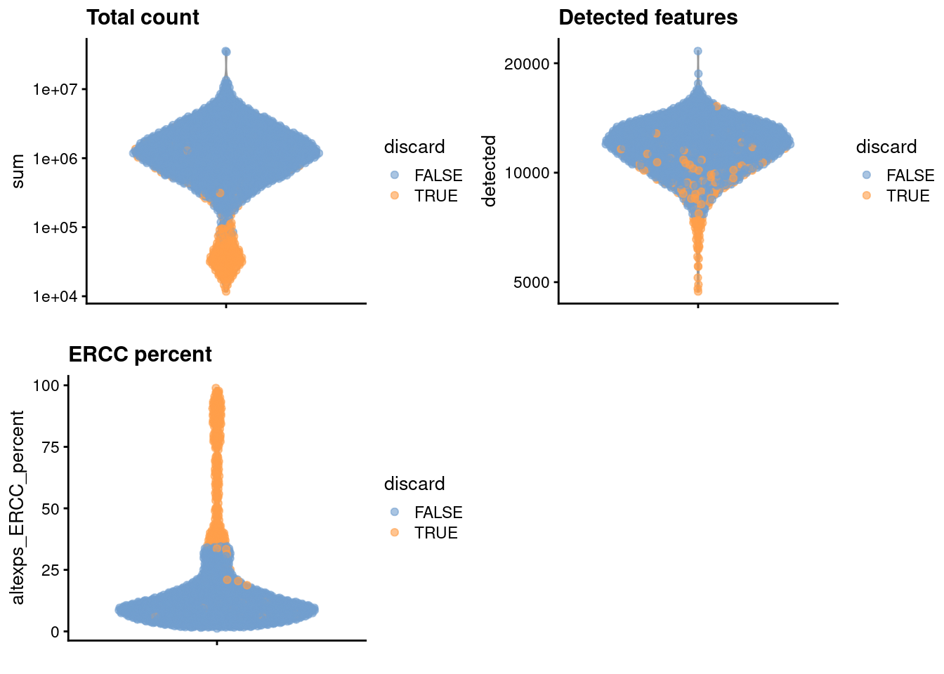
For some reason, no mitochondrial transcripts are available, so we will perform quality control using the spike-in proportions only.
```r
library(scater)
stats <- perCellQCMetrics(sce.nest)
qc <- quickPerCellQC(stats, percent_subsets="altexps_ERCC_percent")
sce.nest <- sce.nest[,!qc$discard]
```
We examine the number of cells discarded for each reason.
```r
colSums(as.matrix(qc))
```
```
## low_lib_size low_n_features high_altexps_ERCC_percent
## 146 28 241
## discard
## 264
```
We create some diagnostic plots for each metric (Figure \@ref(fig:unref-nest-qc-dist)).
```r
colData(unfiltered) <- cbind(colData(unfiltered), stats)
unfiltered$discard <- qc$discard
gridExtra::grid.arrange(
plotColData(unfiltered, y="sum", colour_by="discard") +
scale_y_log10() + ggtitle("Total count"),
plotColData(unfiltered, y="detected", colour_by="discard") +
scale_y_log10() + ggtitle("Detected features"),
plotColData(unfiltered, y="altexps_ERCC_percent",
colour_by="discard") + ggtitle("ERCC percent"),
ncol=2
)
```
(\#fig:unref-nest-qc-dist)Distribution of each QC metric across cells in the Nestorowa HSC dataset. Each point represents a cell and is colored according to whether that cell was discarded.
## Normalization
```r
library(scran)
set.seed(101000110)
clusters <- quickCluster(sce.nest)
sce.nest <- computeSumFactors(sce.nest, clusters=clusters)
sce.nest <- logNormCounts(sce.nest)
```
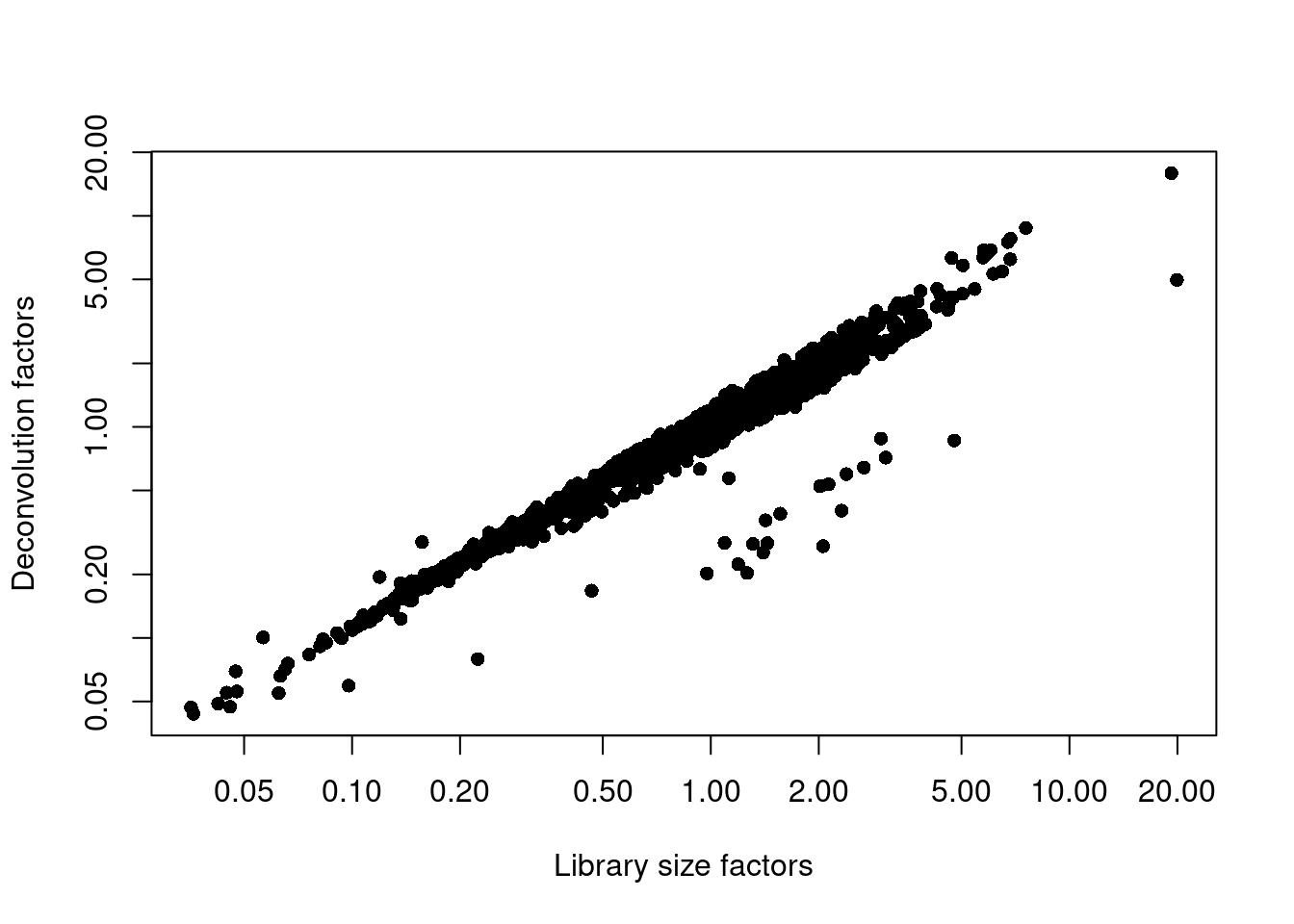
We examine some key metrics for the distribution of size factors, and compare it to the library sizes as a sanity check (Figure \@ref(fig:unref-nest-norm)).
```r
summary(sizeFactors(sce.nest))
```
```
## Min. 1st Qu. Median Mean 3rd Qu. Max.
## 0.044 0.422 0.748 1.000 1.249 15.927
```
```r
plot(librarySizeFactors(sce.nest), sizeFactors(sce.nest), pch=16,
xlab="Library size factors", ylab="Deconvolution factors", log="xy")
```
(\#fig:unref-nest-norm)Relationship between the library size factors and the deconvolution size factors in the Nestorowa HSC dataset.
## Variance modelling
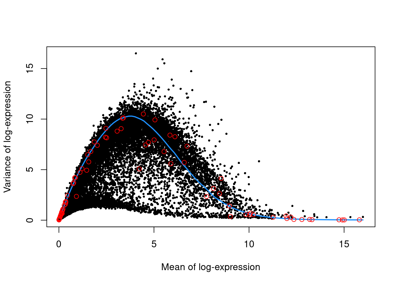
We use the spike-in transcripts to model the technical noise as a function of the mean (Figure \@ref(fig:unref-nest-var)).
```r
set.seed(00010101)
dec.nest <- modelGeneVarWithSpikes(sce.nest, "ERCC")
top.nest <- getTopHVGs(dec.nest, prop=0.1)
```
```r
plot(dec.nest$mean, dec.nest$total, pch=16, cex=0.5,
xlab="Mean of log-expression", ylab="Variance of log-expression")
curfit <- metadata(dec.nest)
curve(curfit$trend(x), col='dodgerblue', add=TRUE, lwd=2)
points(curfit$mean, curfit$var, col="red")
```
(\#fig:unref-nest-var)Per-gene variance as a function of the mean for the log-expression values in the Nestorowa HSC dataset. Each point represents a gene (black) with the mean-variance trend (blue) fitted to the spike-ins (red).
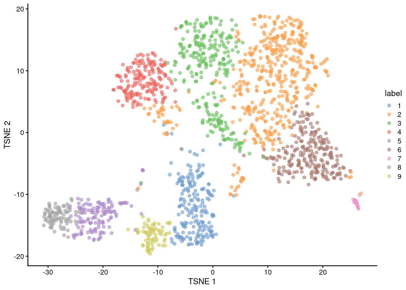
(\#fig:unref-nest-tsne)Obligatory $t$-SNE plot of the Nestorowa HSC dataset, where each point represents a cell and is colored according to the assigned cluster.
## Marker gene detection
```r
markers <- findMarkers(sce.nest, colLabels(sce.nest),
test.type="wilcox", direction="up", lfc=0.5,
row.data=rowData(sce.nest)[,"SYMBOL",drop=FALSE])
```
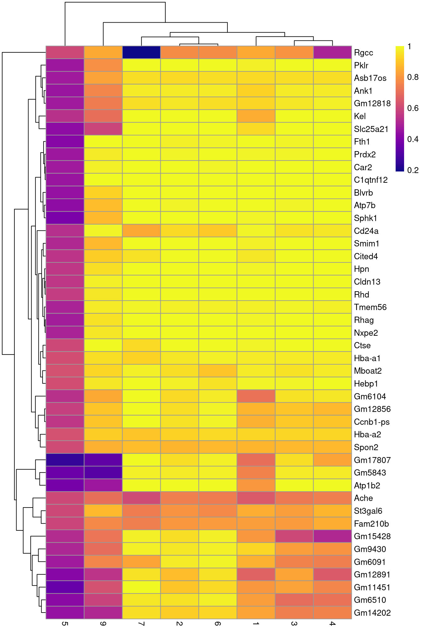
To illustrate the manual annotation process, we examine the marker genes for one of the clusters.
Upregulation of _Car2_, _Hebp1_ amd hemoglobins indicates that cluster 8 contains erythroid precursors.
```r
chosen <- markers[['8']]
best <- chosen[chosen$Top <= 10,]
aucs <- getMarkerEffects(best, prefix="AUC")
rownames(aucs) <- best$SYMBOL
library(pheatmap)
pheatmap(aucs, color=viridis::plasma(100))
```
(\#fig:unref-heat-nest-markers)Heatmap of the AUCs for the top marker genes in cluster 8 compared to all other clusters.
## Cell type annotation
```r
library(SingleR)
mm.ref <- MouseRNAseqData()
# Renaming to symbols to match with reference row names.
renamed <- sce.nest
rownames(renamed) <- uniquifyFeatureNames(rownames(renamed),
rowData(sce.nest)$SYMBOL)
labels <- SingleR(renamed, mm.ref, labels=mm.ref$label.fine)
```
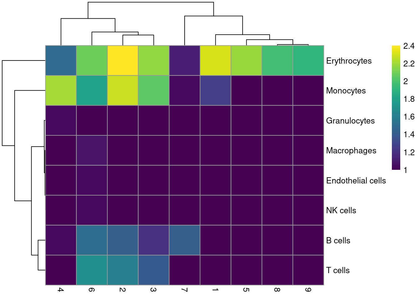
Most clusters are not assigned to any single lineage (Figure \@ref(fig:unref-assignments-nest)), which is perhaps unsurprising given that HSCs are quite different from their terminal fates.
Cluster 8 is considered to contain erythrocytes, which is roughly consistent with our conclusions from the marker gene analysis above.
```r
tab <- table(labels$labels, colLabels(sce.nest))
pheatmap(log10(tab+10), color=viridis::viridis(100))
```
(\#fig:unref-assignments-nest)Heatmap of the distribution of cells for each cluster in the Nestorowa HSC dataset, based on their assignment to each label in the mouse RNA-seq references from the _SingleR_ package.
## Miscellaneous analyses
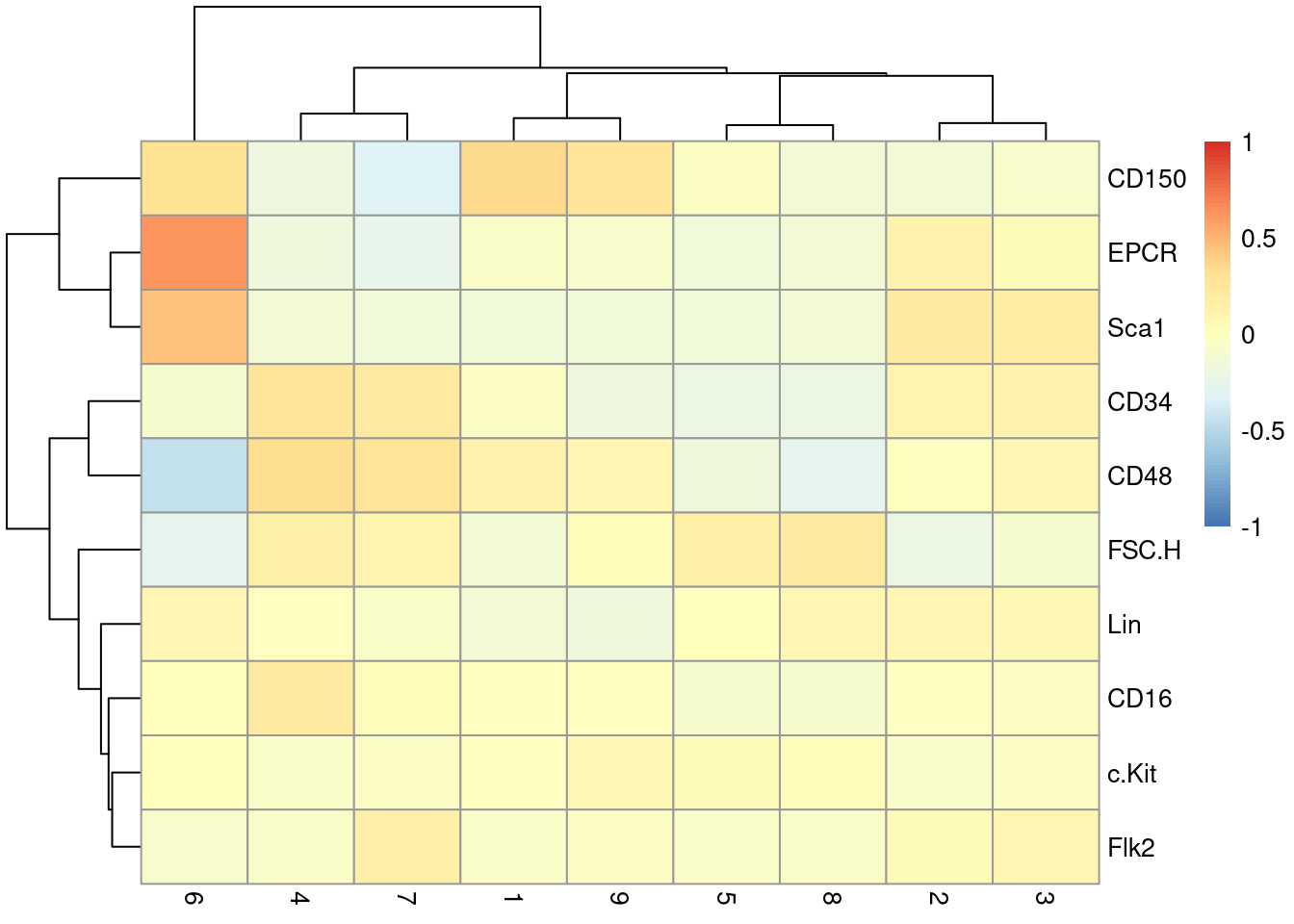
This dataset also contains information about the protein abundances in each cell from FACS.
There is barely any heterogeneity in the chosen markers across the clusters (Figure \@ref(fig:unref-nest-facs));
this is perhaps unsurprising given that all cells should be HSCs of some sort.
```r
Y <- colData(sce.nest)$FACS
keep <- rowSums(is.na(Y))==0 # Removing NA intensities.
se.averaged <- sumCountsAcrossCells(t(Y[keep,]),
colLabels(sce.nest)[keep], average=TRUE)
averaged <- assay(se.averaged)
log.intensities <- log2(averaged+1)
centered <- log.intensities - rowMeans(log.intensities)
pheatmap(centered, breaks=seq(-1, 1, length.out=101))
```
(\#fig:unref-nest-facs)Heatmap of the centered log-average intensity for each target protein quantified by FACS in the Nestorowa HSC dataset.