# Bach mouse mammary gland (10X Genomics)

<script>
document.addEventListener("click", function (event) {
    if (event.target.classList.contains("rebook-collapse")) {
        event.target.classList.toggle("active");
        var content = event.target.nextElementSibling;
        if (content.style.display === "block") {
            content.style.display = "none";
        } else {
            content.style.display = "block";
        }
    }
})
</script>

<style>
.rebook-collapse {
  background-color: #eee;
  color: #444;
  cursor: pointer;
  padding: 18px;
  width: 100%;
  border: none;
  text-align: left;
  outline: none;
  font-size: 15px;
}

.rebook-content {
  padding: 0 18px;
  display: none;
  overflow: hidden;
  background-color: #f1f1f1;
}
</style>

## Introduction

This performs an analysis of the @bach2017differentiation 10X Genomics dataset,
from which we will consider a single sample of epithelial cells from the mouse mammary gland during gestation.

## Data loading


```r
library(scRNAseq)
sce.mam <- BachMammaryData(samples="G_1")
```


```r
library(scater)
rownames(sce.mam) <- uniquifyFeatureNames(
    rowData(sce.mam)$Ensembl, rowData(sce.mam)$Symbol)

library(AnnotationHub)
ens.mm.v97 <- AnnotationHub()[["AH73905"]]
rowData(sce.mam)$SEQNAME <- mapIds(ens.mm.v97, keys=rowData(sce.mam)$Ensembl,
    keytype="GENEID", column="SEQNAME")
```

## Quality control


```r
unfiltered <- sce.mam
```


```r
is.mito <- rowData(sce.mam)$SEQNAME == "MT"
stats <- perCellQCMetrics(sce.mam, subsets=list(Mito=which(is.mito)))
qc <- quickPerCellQC(stats, percent_subsets="subsets_Mito_percent")
sce.mam <- sce.mam[,!qc$discard]
```


```r
colData(unfiltered) <- cbind(colData(unfiltered), stats)
unfiltered$discard <- qc$discard

gridExtra::grid.arrange(
    plotColData(unfiltered, y="sum", colour_by="discard") + 
        scale_y_log10() + ggtitle("Total count"),
    plotColData(unfiltered, y="detected", colour_by="discard") + 
        scale_y_log10() + ggtitle("Detected features"),
    plotColData(unfiltered, y="subsets_Mito_percent", 
        colour_by="discard") + ggtitle("Mito percent"),
    ncol=2
)
```

<div class="figure">
<img src="bach-mammary_files/figure-html/unref-bach-qc-dist-1.png" alt="Distribution of each QC metric across cells in the Bach mammary gland dataset. Each point represents a cell and is colored according to whether that cell was discarded." width="672" />
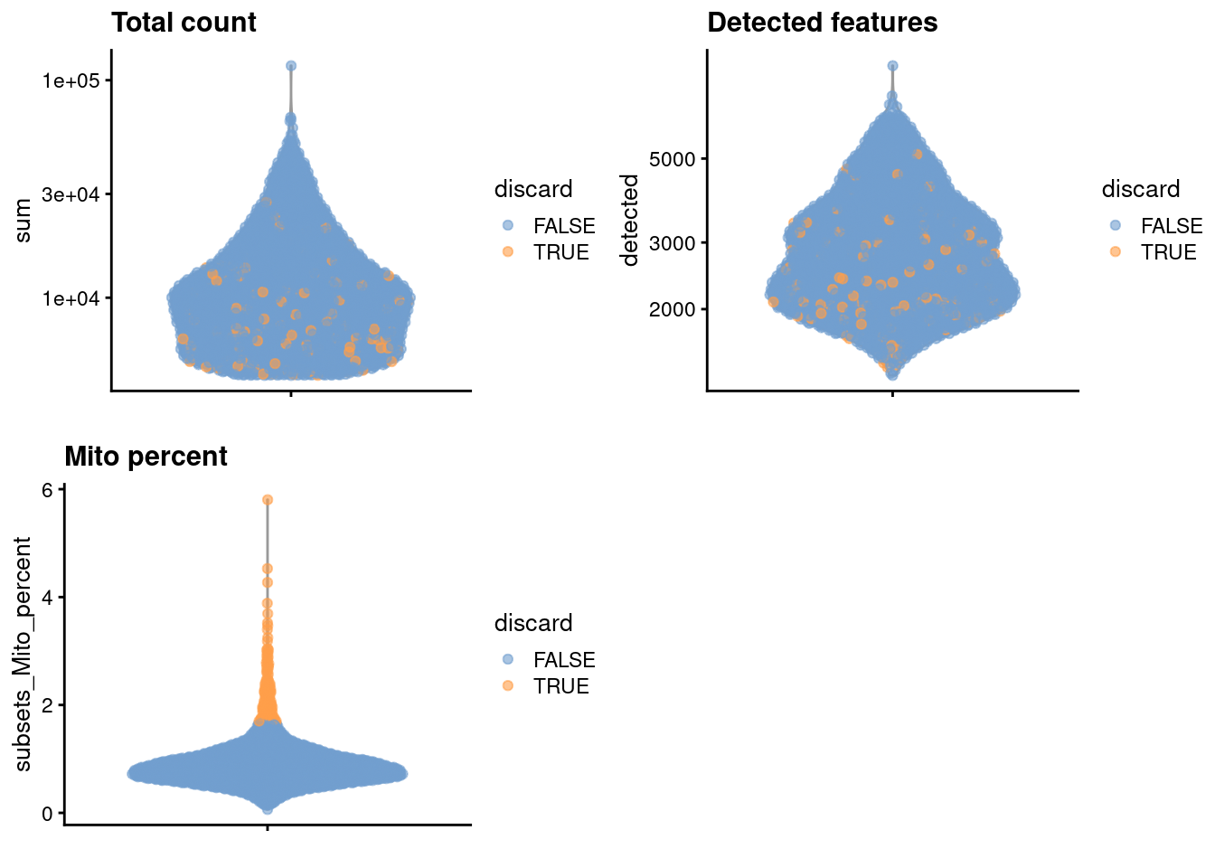
<p class="caption">(\#fig:unref-bach-qc-dist)Distribution of each QC metric across cells in the Bach mammary gland dataset. Each point represents a cell and is colored according to whether that cell was discarded.</p>
</div>


```r
plotColData(unfiltered, x="sum", y="subsets_Mito_percent", 
    colour_by="discard") + scale_x_log10()
```

<div class="figure">
<img src="bach-mammary_files/figure-html/unref-bach-qc-comp-1.png" alt="Percentage of mitochondrial reads in each cell in the Bach mammary gland dataset compared to its total count. Each point represents a cell and is colored according to whether that cell was discarded." width="672" />
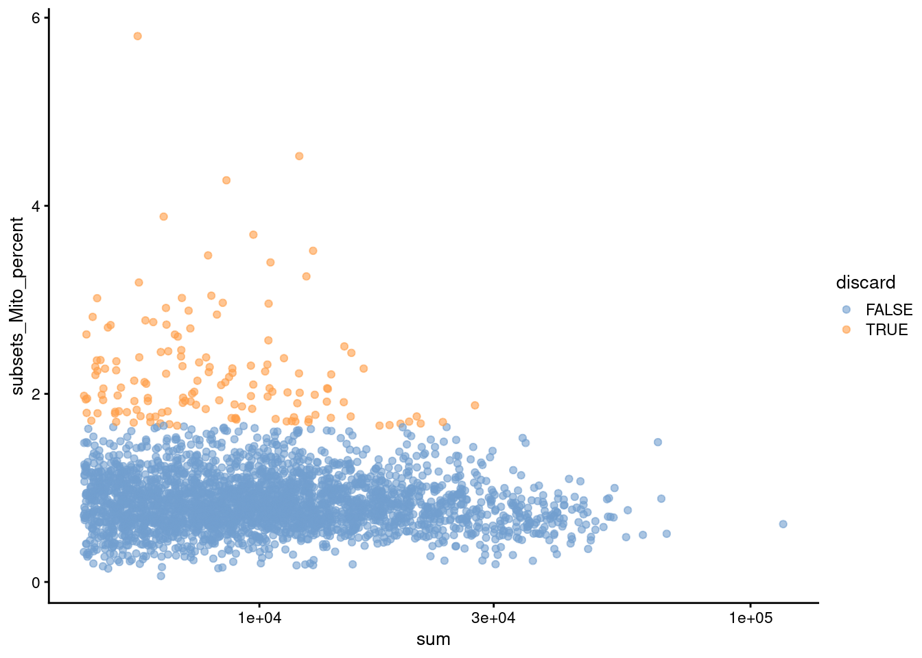
<p class="caption">(\#fig:unref-bach-qc-comp)Percentage of mitochondrial reads in each cell in the Bach mammary gland dataset compared to its total count. Each point represents a cell and is colored according to whether that cell was discarded.</p>
</div>


```r
colSums(as.matrix(qc))
```

```
##              low_lib_size            low_n_features high_subsets_Mito_percent 
##                         0                         0                       143 
##                   discard 
##                       143
```

## Normalization 


```r
library(scran)
set.seed(101000110)
clusters <- quickCluster(sce.mam)
sce.mam <- computeSumFactors(sce.mam, clusters=clusters)
sce.mam <- logNormCounts(sce.mam)
```


```r
summary(sizeFactors(sce.mam))
```

```
##    Min. 1st Qu.  Median    Mean 3rd Qu.    Max. 
##   0.271   0.522   0.758   1.000   1.204  10.958
```


```r
plot(librarySizeFactors(sce.mam), sizeFactors(sce.mam), pch=16,
    xlab="Library size factors", ylab="Deconvolution factors", log="xy")
```

<div class="figure">
<img src="bach-mammary_files/figure-html/unref-bach-norm-1.png" alt="Relationship between the library size factors and the deconvolution size factors in the Bach mammary gland dataset." width="672" />
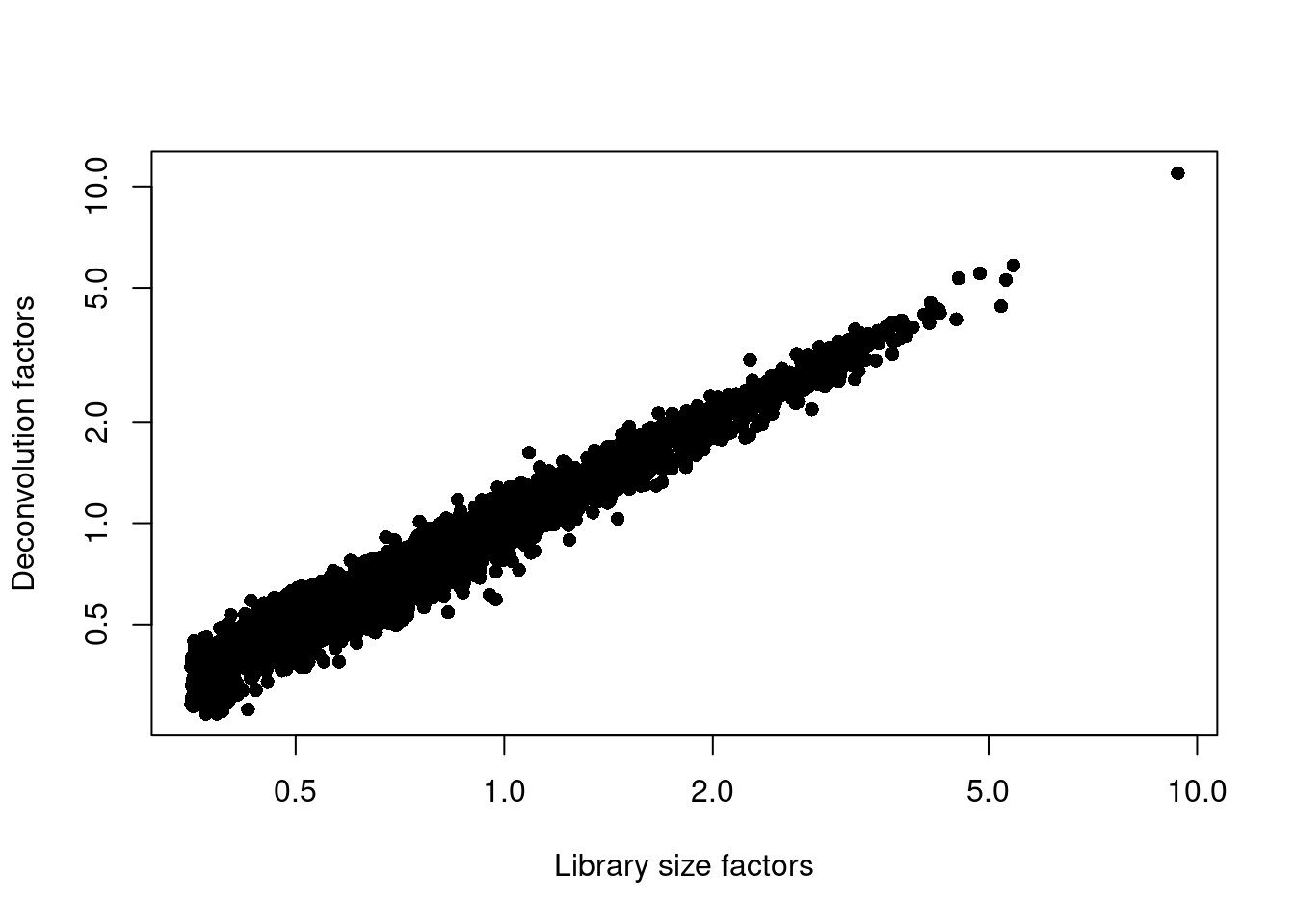
<p class="caption">(\#fig:unref-bach-norm)Relationship between the library size factors and the deconvolution size factors in the Bach mammary gland dataset.</p>
</div>

## Variance modelling

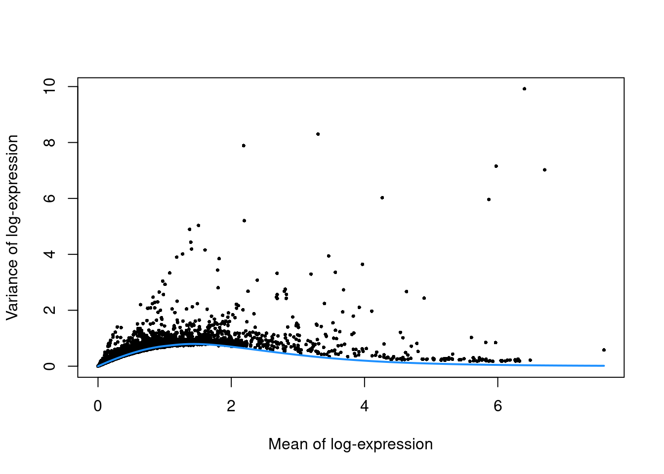
We use a Poisson-based technical trend to capture more genuine biological variation in the biological component.


```r
set.seed(00010101)
dec.mam <- modelGeneVarByPoisson(sce.mam)
top.mam <- getTopHVGs(dec.mam, prop=0.1)
```


```r
plot(dec.mam$mean, dec.mam$total, pch=16, cex=0.5,
    xlab="Mean of log-expression", ylab="Variance of log-expression")
curfit <- metadata(dec.mam)
curve(curfit$trend(x), col='dodgerblue', add=TRUE, lwd=2)
```

<div class="figure">
<img src="bach-mammary_files/figure-html/unref-bach-var-1.png" alt="Per-gene variance as a function of the mean for the log-expression values in the Bach mammary gland dataset. Each point represents a gene (black) with the mean-variance trend (blue) fitted to simulated Poisson counts." width="672" />
<p class="caption">(\#fig:unref-bach-var)Per-gene variance as a function of the mean for the log-expression values in the Bach mammary gland dataset. Each point represents a gene (black) with the mean-variance trend (blue) fitted to simulated Poisson counts.</p>
</div>

## Dimensionality reduction


```r
library(BiocSingular)
set.seed(101010011)
sce.mam <- denoisePCA(sce.mam, technical=dec.mam, subset.row=top.mam)
sce.mam <- runTSNE(sce.mam, dimred="PCA")
```


```r
ncol(reducedDim(sce.mam, "PCA"))
```

```
## [1] 15
```

## Clustering 

We use a higher `k` to obtain coarser clusters (for use in `doubletCluster()` later).


```r
snn.gr <- buildSNNGraph(sce.mam, use.dimred="PCA", k=25)
colLabels(sce.mam) <- factor(igraph::cluster_walktrap(snn.gr)$membership)
```


```r
table(colLabels(sce.mam))
```

```
## 
##   1   2   3   4   5   6   7   8   9  10 
## 550 799 716 452  24  84  52  39  32  24
```


```r
plotTSNE(sce.mam, colour_by="label")
```

<div class="figure">
<img src="bach-mammary_files/figure-html/unref-bach-tsne-1.png" alt="Obligatory $t$-SNE plot of the Bach mammary gland dataset, where each point represents a cell and is colored according to the assigned cluster." width="672" />
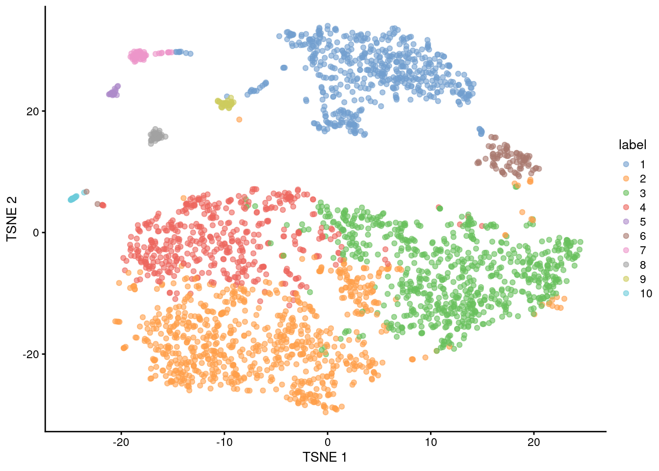
<p class="caption">(\#fig:unref-bach-tsne)Obligatory $t$-SNE plot of the Bach mammary gland dataset, where each point represents a cell and is colored according to the assigned cluster.</p>
</div>

## Session Info {-}

<button class="rebook-collapse">View session info</button>
<div class="rebook-content">
```
R version 4.3.1 (2023-06-16)
Platform: x86_64-pc-linux-gnu (64-bit)
Running under: Ubuntu 22.04.3 LTS

Matrix products: default
BLAS:   /home/biocbuild/bbs-3.18-bioc/R/lib/libRblas.so 
LAPACK: /usr/lib/x86_64-linux-gnu/lapack/liblapack.so.3.10.0

locale:
 [1] LC_CTYPE=en_US.UTF-8       LC_NUMERIC=C              
 [3] LC_TIME=en_GB              LC_COLLATE=C              
 [5] LC_MONETARY=en_US.UTF-8    LC_MESSAGES=en_US.UTF-8   
 [7] LC_PAPER=en_US.UTF-8       LC_NAME=C                 
 [9] LC_ADDRESS=C               LC_TELEPHONE=C            
[11] LC_MEASUREMENT=en_US.UTF-8 LC_IDENTIFICATION=C       

time zone: America/New_York
tzcode source: system (glibc)

attached base packages:
[1] stats4    stats     graphics  grDevices utils     datasets  methods  
[8] base     

other attached packages:
 [1] BiocSingular_1.18.0         scran_1.30.0               
 [3] AnnotationHub_3.10.0        BiocFileCache_2.10.0       
 [5] dbplyr_2.3.4                scater_1.30.0              
 [7] ggplot2_3.4.4               scuttle_1.12.0             
 [9] ensembldb_2.26.0            AnnotationFilter_1.26.0    
[11] GenomicFeatures_1.54.0      AnnotationDbi_1.64.0       
[13] Matrix_1.6-1.1              scRNAseq_2.15.0            
[15] SingleCellExperiment_1.24.0 SummarizedExperiment_1.32.0
[17] Biobase_2.62.0              GenomicRanges_1.54.0       
[19] GenomeInfoDb_1.38.0         IRanges_2.36.0             
[21] S4Vectors_0.40.0            BiocGenerics_0.48.0        
[23] MatrixGenerics_1.14.0       matrixStats_1.0.0          
[25] BiocStyle_2.30.0            rebook_1.12.0              

loaded via a namespace (and not attached):
  [1] rstudioapi_0.15.0             jsonlite_1.8.7               
  [3] CodeDepends_0.6.5             magrittr_2.0.3               
  [5] ggbeeswarm_0.7.2              farver_2.1.1                 
  [7] rmarkdown_2.25                BiocIO_1.12.0                
  [9] zlibbioc_1.48.0               vctrs_0.6.4                  
 [11] memoise_2.0.1                 Rsamtools_2.18.0             
 [13] DelayedMatrixStats_1.24.0     RCurl_1.98-1.12              
 [15] htmltools_0.5.6.1             S4Arrays_1.2.0               
 [17] progress_1.2.2                curl_5.1.0                   
 [19] BiocNeighbors_1.20.0          SparseArray_1.2.0            
 [21] sass_0.4.7                    bslib_0.5.1                  
 [23] cachem_1.0.8                  GenomicAlignments_1.38.0     
 [25] igraph_1.5.1                  mime_0.12                    
 [27] lifecycle_1.0.3               pkgconfig_2.0.3              
 [29] rsvd_1.0.5                    R6_2.5.1                     
 [31] fastmap_1.1.1                 GenomeInfoDbData_1.2.11      
 [33] shiny_1.7.5.1                 digest_0.6.33                
 [35] colorspace_2.1-0              dqrng_0.3.1                  
 [37] irlba_2.3.5.1                 ExperimentHub_2.10.0         
 [39] RSQLite_2.3.1                 beachmat_2.18.0              
 [41] labeling_0.4.3                filelock_1.0.2               
 [43] fansi_1.0.5                   httr_1.4.7                   
 [45] abind_1.4-5                   compiler_4.3.1               
 [47] bit64_4.0.5                   withr_2.5.1                  
 [49] BiocParallel_1.36.0           viridis_0.6.4                
 [51] DBI_1.1.3                     biomaRt_2.58.0               
 [53] rappdirs_0.3.3                DelayedArray_0.28.0          
 [55] bluster_1.12.0                rjson_0.2.21                 
 [57] tools_4.3.1                   vipor_0.4.5                  
 [59] beeswarm_0.4.0                interactiveDisplayBase_1.40.0
 [61] httpuv_1.6.12                 glue_1.6.2                   
 [63] restfulr_0.0.15               promises_1.2.1               
 [65] grid_4.3.1                    Rtsne_0.16                   
 [67] cluster_2.1.4                 generics_0.1.3               
 [69] gtable_0.3.4                  hms_1.1.3                    
 [71] metapod_1.10.0                ScaledMatrix_1.10.0          
 [73] xml2_1.3.5                    utf8_1.2.4                   
 [75] XVector_0.42.0                ggrepel_0.9.4                
 [77] BiocVersion_3.18.0            pillar_1.9.0                 
 [79] stringr_1.5.0                 limma_3.58.0                 
 [81] later_1.3.1                   dplyr_1.1.3                  
 [83] lattice_0.22-5                rtracklayer_1.62.0           
 [85] bit_4.0.5                     tidyselect_1.2.0             
 [87] locfit_1.5-9.8                Biostrings_2.70.0            
 [89] knitr_1.44                    gridExtra_2.3                
 [91] bookdown_0.36                 ProtGenerics_1.34.0          
 [93] edgeR_4.0.0                   xfun_0.40                    
 [95] statmod_1.5.0                 stringi_1.7.12               
 [97] lazyeval_0.2.2                yaml_2.3.7                   
 [99] evaluate_0.22                 codetools_0.2-19             
[101] tibble_3.2.1                  BiocManager_1.30.22          
[103] graph_1.80.0                  cli_3.6.1                    
[105] xtable_1.8-4                  munsell_0.5.0                
[107] jquerylib_0.1.4               Rcpp_1.0.11                  
[109] dir.expiry_1.10.0             png_0.1-8                    
[111] XML_3.99-0.14                 parallel_4.3.1               
[113] ellipsis_0.3.2                blob_1.2.4                   
[115] prettyunits_1.2.0             sparseMatrixStats_1.14.0     
[117] bitops_1.0-7                  viridisLite_0.4.2            
[119] scales_1.2.1                  purrr_1.0.2                  
[121] crayon_1.5.2                  rlang_1.1.1                  
[123] cowplot_1.1.1                 KEGGREST_1.42.0              
```
</div>