---
bibliography: ref.bib
---
# CBP, wild-type versus knock-out
## Background
Here, we perform a window-based DB analysis to identify differentially bound (DB) regions for CREB-binding protein (CBP).
This particular dataset comes from a study comparing wild-type (WT) and CBP knock-out (KO) animals [@kasper2014genomewide], with two biological replicates for each genotype.
As before, we obtain the BAM files and indices from *[chipseqDBData](https://bioconductor.org/packages/3.19/chipseqDBData)*.
```r
library(chipseqDBData)
cbpdata <- CBPData()
cbpdata
```
```
## DataFrame with 4 rows and 3 columns
## Name Description Path
##
## 1 SRR1145787 CBP wild-type (1)
## 2 SRR1145788 CBP wild-type (2)
## 3 SRR1145789 CBP knock-out (1)
## 4 SRR1145790 CBP knock-out (2)
```
## Pre-processing
We check some mapping statistics for the CBP dataset with *[Rsamtools](https://bioconductor.org/packages/3.19/Rsamtools)*, as previously described.
```r
library(Rsamtools)
diagnostics <- list()
for (b in seq_along(cbpdata$Path)) {
bam <- cbpdata$Path[[b]]
total <- countBam(bam)$records
mapped <- countBam(bam, param=ScanBamParam(
flag=scanBamFlag(isUnmapped=FALSE)))$records
marked <- countBam(bam, param=ScanBamParam(
flag=scanBamFlag(isUnmapped=FALSE, isDuplicate=TRUE)))$records
diagnostics[[b]] <- c(Total=total, Mapped=mapped, Marked=marked)
}
diag.stats <- data.frame(do.call(rbind, diagnostics))
rownames(diag.stats) <- cbpdata$Name
diag.stats$Prop.mapped <- diag.stats$Mapped/diag.stats$Total*100
diag.stats$Prop.marked <- diag.stats$Marked/diag.stats$Mapped*100
diag.stats
```
```
## Total Mapped Marked Prop.mapped Prop.marked
## SRR1145787 28525952 24289396 2022868 85.15 8.328
## SRR1145788 25514465 21604007 1939224 84.67 8.976
## SRR1145789 34476967 29195883 2412650 84.68 8.264
## SRR1145790 32624587 27348488 2617879 83.83 9.572
```
We construct a `readParam` object to standardize the parameter settings in this analysis.
The ENCODE blacklist is again used to remove reads in problematic regions [@dunham2012].
```r
library(BiocFileCache)
bfc <- BiocFileCache("local", ask=FALSE)
black.path <- bfcrpath(bfc, file.path("https://www.encodeproject.org",
"files/ENCFF547MET/@@download/ENCFF547MET.bed.gz"))
library(rtracklayer)
blacklist <- import(black.path)
```
We set the minimum mapping quality score to 10 to remove poorly or non-uniquely aligned reads.
```r
library(csaw)
param <- readParam(minq=10, discard=blacklist)
param
```
```
## Extracting reads in single-end mode
## Duplicate removal is turned off
## Minimum allowed mapping score is 10
## Reads are extracted from both strands
## No restrictions are placed on read extraction
## Reads in 164 regions will be discarded
```
## Quantifying coverage
### Computing the average fragment length
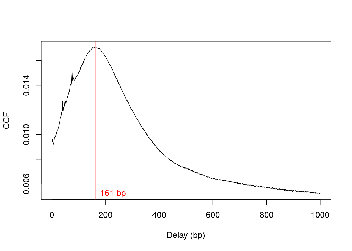
The average fragment length is estimated by maximizing the cross-correlation function (Figure \@ref(fig:cbp-ccfplot)), as previously described.
Generally, cross-correlations for TF datasets are sharper than for histone marks as the TFs typically contact a smaller genomic interval.
This results in more pronounced strand bimodality in the binding profile.
```r
x <- correlateReads(cbpdata$Path, param=reform(param, dedup=TRUE))
frag.len <- maximizeCcf(x)
frag.len
```
```
## [1] 161
```
```r
plot(1:length(x)-1, x, xlab="Delay (bp)", ylab="CCF", type="l")
abline(v=frag.len, col="red")
text(x=frag.len, y=min(x), paste(frag.len, "bp"), pos=4, col="red")
```
(\#fig:cbp-ccfplot)Cross-correlation function (CCF) against delay distance for the CBP dataset. The delay with the maximum correlation is shown as the red line.
### Counting reads into windows
Reads are then counted into sliding windows using *[csaw](https://bioconductor.org/packages/3.19/csaw)* [@lun2016csaw].
For TF data analyses, smaller windows are necessary to capture sharp binding sites.
A large window size will be suboptimal as the count for a particular site will be "contaminated" by non-specific background in the neighbouring regions.
In this case, a window size of 10 bp is used.
```r
win.data <- windowCounts(cbpdata$Path, param=param, width=10, ext=frag.len)
win.data
```
```
## class: RangedSummarizedExperiment
## dim: 9952827 4
## metadata(6): spacing width ... param final.ext
## assays(1): counts
## rownames: NULL
## rowData names(0):
## colnames: NULL
## colData names(4): bam.files totals ext rlen
```
The default spacing of 50 bp is also used here.
This may seem inappropriate given that the windows are only 10 bp.
However, reads lying in the interval between adjacent windows will still be counted into several windows.
This is because reads are extended to the value of `frag.len`, which is substantially larger than the 50 bp spacing^[Smaller spacings can be used but will provide little benefit given that each extended read already overlaps multiple windows.].
## Filtering of low-abundance windows
We remove low-abundance windows by computing the coverage in each window relative to a global estimate of background enrichment (Section \@ref(sec:global-filter)).
The majority of windows in background regions are filtered out upon applying a modest fold-change threshold.
This leaves a small set of relevant windows for further analysis.
```r
bins <- windowCounts(cbpdata$Path, bin=TRUE, width=10000, param=param)
filter.stat <- filterWindowsGlobal(win.data, bins)
min.fc <- 3
keep <- filter.stat$filter > log2(min.fc)
summary(keep)
```
```
## Mode FALSE TRUE
## logical 9652836 299991
```
```r
filtered.data <- win.data[keep,]
```
Note that the 10 kbp bins are used here for filtering, while smaller 2 kbp bins were used in the corresponding step for the H3K9ac analysis.
This is purely for convenience -- the 10 kbp counts for this dataset were previously loaded for normalization, and can be re-used during filtering to save time.
Changes in bin size will have little impact on the results, so long as the bins (and their counts) are large enough for precise estimation of the background abundance.
While smaller bins provide greater spatial resolution, this is irrelevant for quantifying coverage in large background regions that span most of the genome.
## Normalization for composition biases
We expect unbalanced DB in this dataset as CBP function should be compromised in the KO cells,
such that most - if not all - of the DB sites should exhibit increased CBP binding in the WT condition.
To remove this bias, we assign reads to large genomic bins and assume that most bins represent non-DB background regions [@lun2014].
Any systematic differences in the coverage of those bins is attributed to composition bias and is normalized out.
Specifically, the trimmed mean of M-values (TMM) method [@oshlack2010] is applied to compute normalization factors from the bin counts.
These factors are stored in `win.data`^[See the `se.out=` argument.] so that they will be applied during the DB analysis with the window counts.
```r
win.data <- normFactors(bins, se.out=win.data)
(normfacs <- win.data$norm.factors)
```
```
## [1] 1.0126 0.9083 1.0444 1.0411
```
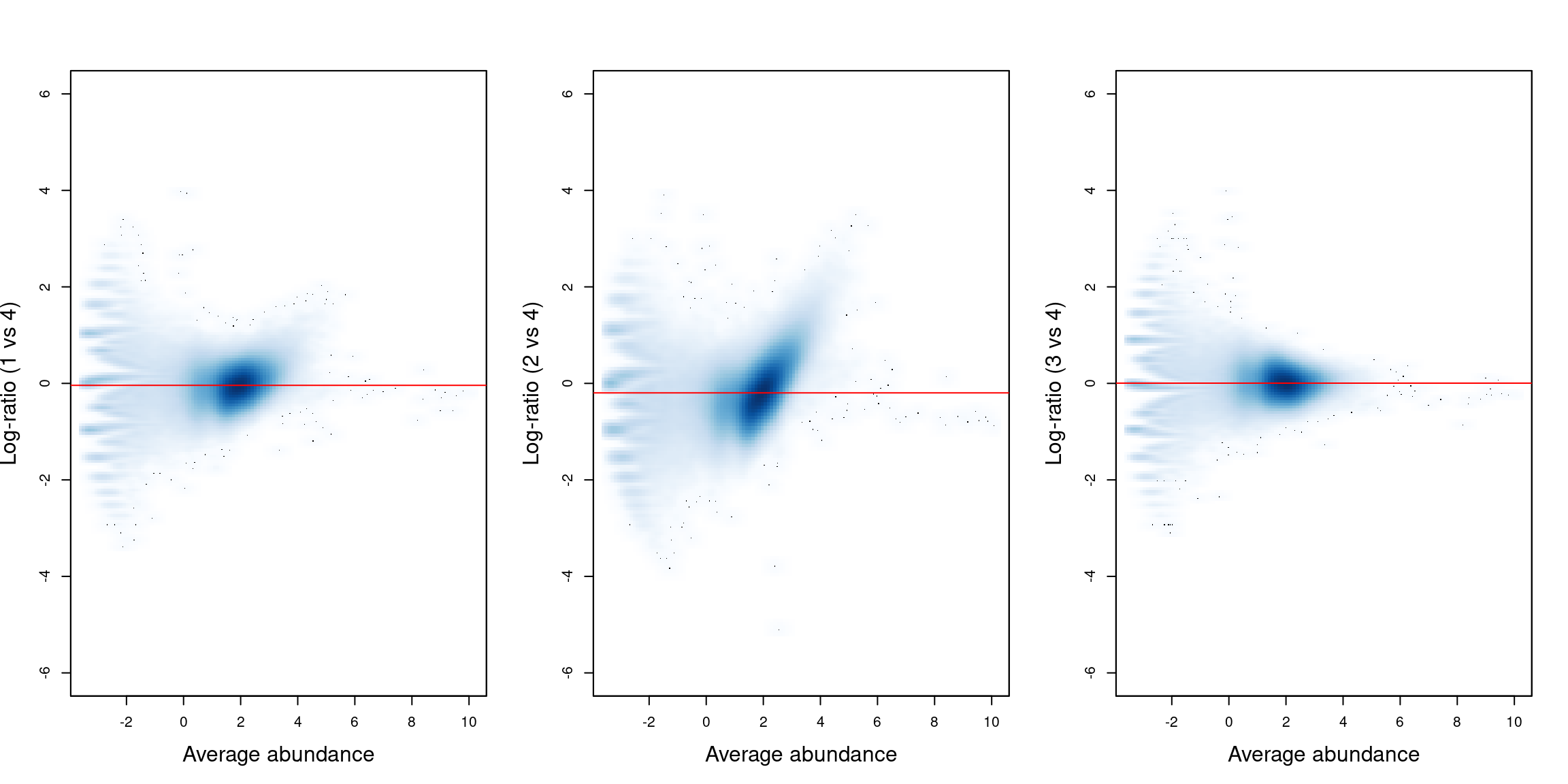
We visualize the effect of normalization with mean-difference plots between pairs of samples (Figure \@ref(fig:cbp-compoplot)).
The dense cloud in each plot represents the majority of bins in the genome.
These are assumed to mostly contain background regions.
A non-zero log-fold change for these bins indicates that composition bias is present between samples.
The red line represents the log-ratio of normalization factors and passes through the centre of the cloud in each plot,
indicating that the bias has been successfully identified and removed.
```r
bin.ab <- scaledAverage(bins)
adjc <- calculateCPM(bins, use.norm.factors=FALSE)
par(cex.lab=1.5, mfrow=c(1,3))
smoothScatter(bin.ab, adjc[,1]-adjc[,4], ylim=c(-6, 6),
xlab="Average abundance", ylab="Log-ratio (1 vs 4)")
abline(h=log2(normfacs[1]/normfacs[4]), col="red")
smoothScatter(bin.ab, adjc[,2]-adjc[,4], ylim=c(-6, 6),
xlab="Average abundance", ylab="Log-ratio (2 vs 4)")
abline(h=log2(normfacs[2]/normfacs[4]), col="red")
smoothScatter(bin.ab, adjc[,3]-adjc[,4], ylim=c(-6, 6),
xlab="Average abundance", ylab="Log-ratio (3 vs 4)")
abline(h=log2(normfacs[3]/normfacs[4]), col="red")
```
(\#fig:cbp-compoplot)Mean-difference plots for the bin counts, comparing sample 4 to all other samples. The red line represents the log-ratio of the normalization factors between samples.
Note that this normalization strategy is quite different from that in the H3K9ac analysis.
Here, systematic DB in one direction is expected between conditions, given that CBP function is lost in the KO genotype.
This means that the assumption of a non-DB majority (required for non-linear normalization of the H3K9ac data) is not valid.
No such assumption is made by the binned-TMM approach described above, which makes it more appropriate for use in the CBP analysis.
## Statistical modelling {#sec:cbp-statistical-modelling}
We model counts for each window using *[edgeR](https://bioconductor.org/packages/3.19/edgeR)* [@mccarthy2012; @robinson2010].
First, we convert our `RangedSummarizedExperiment` object into a `DGEList`.
```r
library(edgeR)
y <- asDGEList(filtered.data)
summary(y)
```
```
## Length Class Mode
## counts 1199964 -none- numeric
## samples 3 data.frame list
```
We then construct a design matrix for our experimental design.
Again, we have a simple one-way layout with two groups of two replicates.
```r
genotype <- cbpdata$Description
genotype[grep("wild-type", genotype)] <- "wt"
genotype[grep("knock-out", genotype)] <- "ko"
genotype <- factor(genotype)
design <- model.matrix(~0+genotype)
colnames(design) <- levels(genotype)
design
```
```
## ko wt
## 1 0 1
## 2 0 1
## 3 1 0
## 4 1 0
## attr(,"assign")
## [1] 1 1
## attr(,"contrasts")
## attr(,"contrasts")$genotype
## [1] "contr.treatment"
```
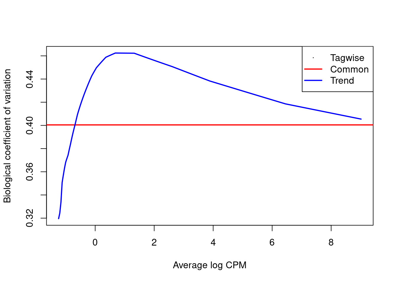
We estimate the negative binomial (NB) and quasi-likelihood (QL) dispersions for each window [@lund2012].
The estimated NB dispersions (Figure \@ref(fig:cbp-bcvplot)) are substantially larger than those observed in the H3K9ac dataset.
They also exhibit an unusual increasing trend with respect to abundance.
```r
y <- estimateDisp(y, design)
summary(y$trended.dispersion)
```
```
## Min. 1st Qu. Median Mean 3rd Qu. Max.
## 0.102 0.129 0.146 0.152 0.176 0.214
```
```r
plotBCV(y)
```
(\#fig:cbp-bcvplot)Abundance-dependent trend in the biological coefficient of variation (i.e., the root-NB dispersion) for each window, represented by the blue line. Common (red) and tagwise estimates (black) are also shown.
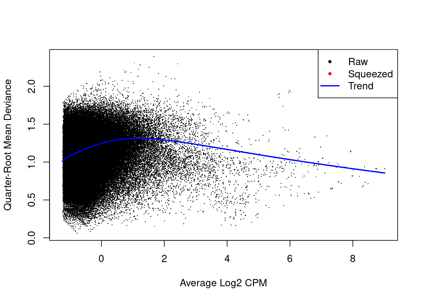
The estimated prior d.f. is also infinite, meaning that all the QL dispersions are equal to the trend (Figure \@ref(fig:cbp-qlplot)).
```r
fit <- glmQLFit(y, design, robust=TRUE)
summary(fit$df.prior)
```
```
## Min. 1st Qu. Median Mean 3rd Qu. Max.
## Inf Inf Inf Inf Inf Inf
```
```r
plotQLDisp(fit)
```
(\#fig:cbp-qlplot)Effect of EB shrinkage on the raw QL dispersion estimate for each window (black) towards the abundance-dependent trend (blue) to obtain squeezed estimates (red). Quarter-root estimates are shown for greater dynamic range.
These results are consistent with the presence of a systematic difference in CBP enrichment between the WT replicates.
An increasing trend in Figure \@ref(fig:cbp-bcvplot) is typical after normalization for composition biases,
where replicates exhibit some differences in efficiency that manifest as increased dispersions at high abundance.
The dispersions for all windows are inflated to a similarly large value by this difference,
manifesting as low variability in the dispersions across windows.
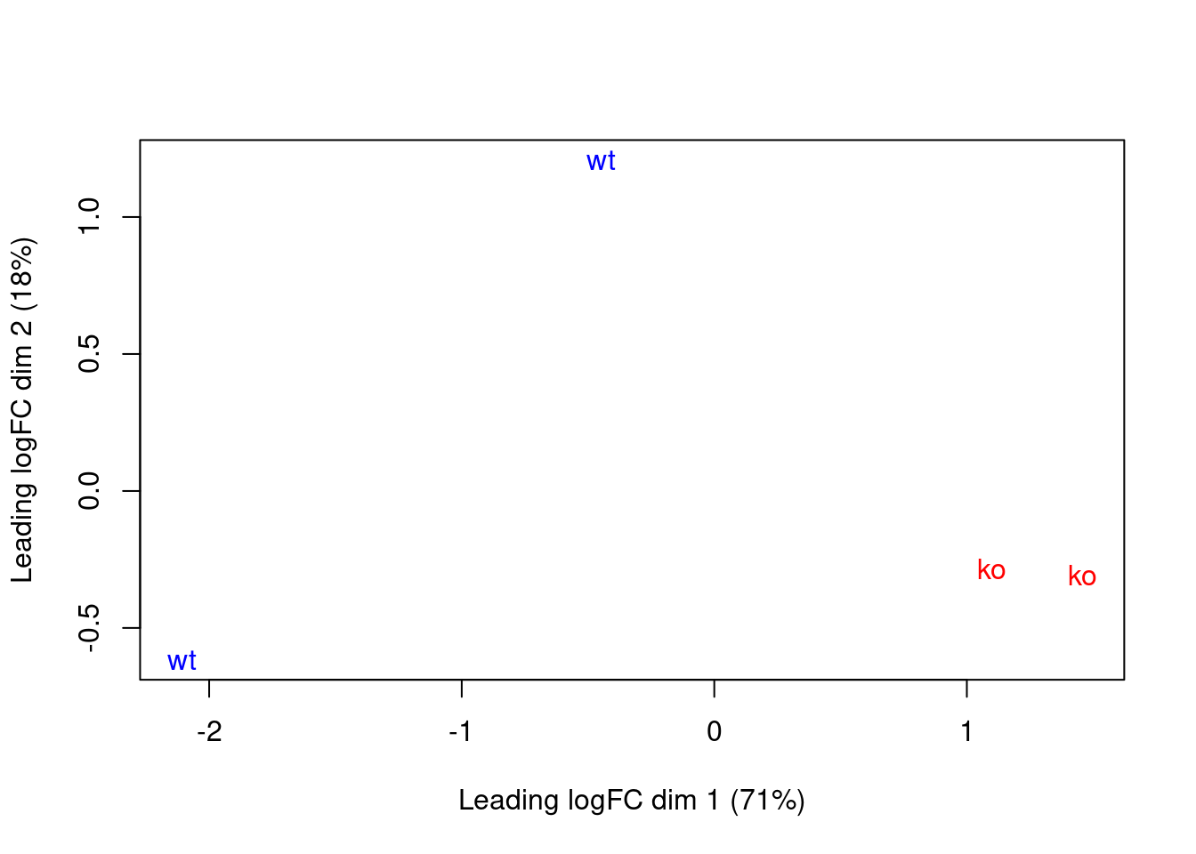
This effect is illustrated in Figure \@ref(fig:cbp-mdsplot) where the WT samples are clearly separated in both dimensions.
```r
plotMDS(cpm(y, log=TRUE), top=10000, labels=genotype,
col=c("red", "blue")[as.integer(genotype)])
```
(\#fig:cbp-mdsplot)MDS plot with two dimensions for all samples in the CBP dataset. Samples are labelled and coloured according to the genotype. A larger top set of windows was used to improve the visualization of the genome-wide differences between the WT samples.
The presence of a large batch effect between replicates is not ideal.
Nonetheless, we can still proceed with the DB analysis - albeit with some loss of power due to the inflated NB dispersions -
given that there are strong differences between genotypes in Figure \@ref(fig:cbp-mdsplot),
## Testing for DB
We test for a significant difference in binding between genotypes in each window using the QL F-test.
```r
contrast <- makeContrasts(wt-ko, levels=design)
res <- glmQLFTest(fit, contrast=contrast)
```
Windows less than 100 bp apart are clustered into regions [@lun2014] with a maximum cluster width of 5 kbp.
We then control the region-level FDR by combining per-window $p$-values using Simes' method [@simes1986].
```r
merged <- mergeResults(filtered.data, res$table, tol=100,
merge.args=list(max.width=5000))
merged$regions
```
```
## GRanges object with 61773 ranges and 0 metadata columns:
## seqnames ranges strand
##
## [1] chr1 3613551-3613610 *
## [2] chr1 4785501-4785860 *
## [3] chr1 4807601-4808010 *
## [4] chr1 4857451-4857910 *
## [5] chr1 4858301-4858460 *
## ... ... ... ...
## [61769] chrY 90808801-90808910 *
## [61770] chrY 90810901-90810910 *
## [61771] chrY 90811301-90811360 *
## [61772] chrY 90811601-90811660 *
## [61773] chrY 90811851-90813910 *
## -------
## seqinfo: 66 sequences from an unspecified genome
```
```r
tabcom <- merged$combined
is.sig <- tabcom$FDR <= 0.05
summary(is.sig)
```
```
## Mode FALSE TRUE
## logical 57912 3861
```
All significant regions have increased CBP binding in the WT genotype.
This is expected given that protein function should be lost in the KO genotype.
```r
table(tabcom$direction[is.sig])
```
```
##
## down up
## 2 3859
```
```r
# Direction according the best window in each cluster.
tabbest <- merged$best
is.sig.pos <- (tabbest$rep.logFC > 0)[is.sig]
summary(is.sig.pos)
```
```
## Mode FALSE TRUE
## logical 2 3859
```
We save the results to file in the form of a serialized R object for later inspection.
```r
out.ranges <- merged$regions
mcols(out.ranges) <- DataFrame(tabcom,
best.pos=mid(ranges(rowRanges(filtered.data[tabbest$rep.test]))),
best.logFC=tabbest$rep.logFC)
saveRDS(file="cbp_results.rds", out.ranges)
```
## Annotation and visualization
We annotate each region using the `detailRanges()` function.
```r
library(TxDb.Mmusculus.UCSC.mm10.knownGene)
library(org.Mm.eg.db)
anno <- detailRanges(out.ranges, orgdb=org.Mm.eg.db,
txdb=TxDb.Mmusculus.UCSC.mm10.knownGene)
mcols(out.ranges) <- cbind(mcols(out.ranges), anno)
```
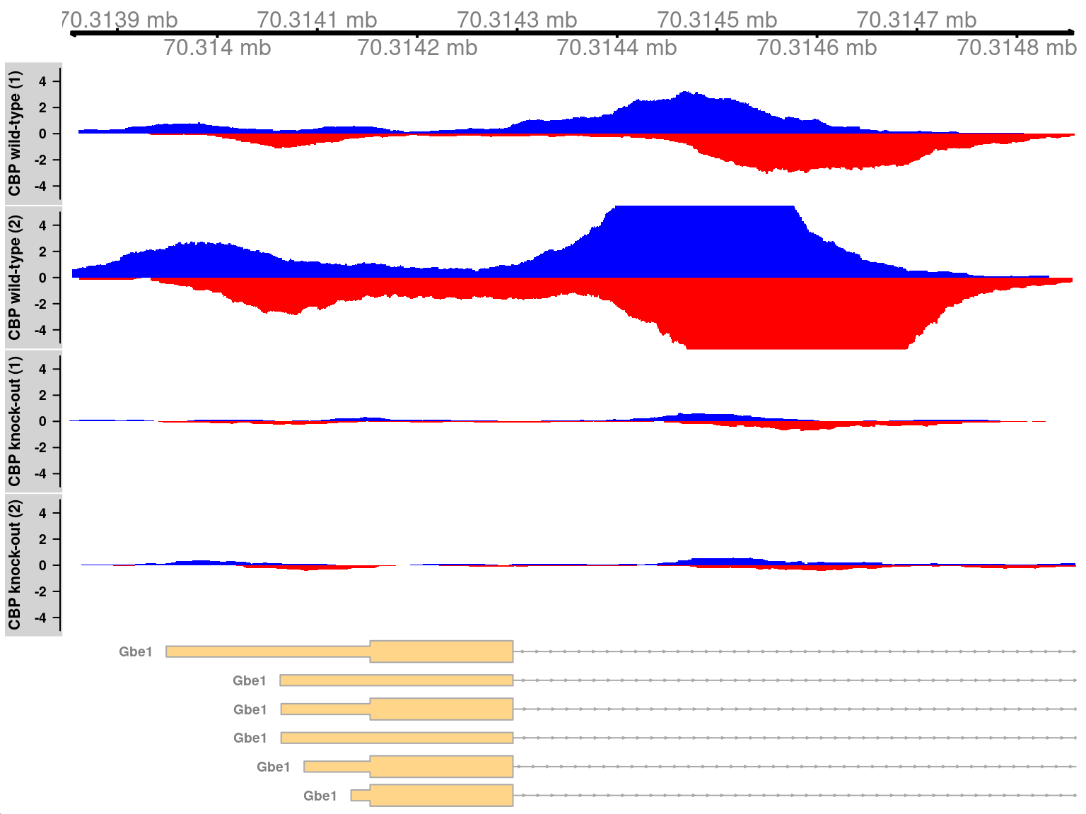
We visualize one of the top-ranked DB regions here.
This corresponds to a simple DB event as all windows are changing in the same direction, i.e., up in the WT.
The binding region is also quite small relative to some of the H3K9ac examples,
consistent with sharp TF binding to a specific recognition site.
```r
o <- order(out.ranges$PValue)
cur.region <- out.ranges[o[2]]
cur.region
```
```
## GRanges object with 1 range and 13 metadata columns:
## seqnames ranges strand | num.tests num.up.logFC num.down.logFC
## |
## [1] chr16 70313851-70314860 * | 21 20 0
## PValue FDR direction rep.test rep.logFC best.pos
##
## [1] 8.71584e-11 2.06063e-06 up 115786 4.48777 70314505
## best.logFC overlap left right
##
## [1] 4.22028 Gbe1:+:PE
## -------
## seqinfo: 66 sequences from an unspecified genome
```
We use *[Gviz](https://bioconductor.org/packages/3.19/Gviz)* [@hahne2016visualizing] to plot the results.
As in the [H3K9ac analysis](https://bioconductor.org/packages/3.19/chipseqDB/vignettes/h3k9ac.html#visualizing-db-results),
we set up some tracks to display genome coordinates and gene annotation.
```r
library(Gviz)
gax <- GenomeAxisTrack(col="black", fontsize=15, size=2)
greg <- GeneRegionTrack(TxDb.Mmusculus.UCSC.mm10.knownGene, showId=TRUE,
geneSymbol=TRUE, name="", background.title="transparent")
symbols <- unlist(mapIds(org.Mm.eg.db, gene(greg), "SYMBOL",
"ENTREZID", multiVals = "first"))
symbol(greg) <- symbols[gene(greg)]
```
We visualize two tracks for each sample -- one for the forward-strand coverage, another for the reverse-strand coverage.
This allows visualization of the strand bimodality that is characteristic of genuine TF binding sites.
In Figure \@ref(fig:cbp-tfplot), two adjacent sites are present at the *Gbe1* promoter, both of which exhibit increased binding in the WT genotype.
Coverage is also substantially different between the WT replicates, consistent with the presence of a batch effect.
```r
collected <- list()
lib.sizes <- filtered.data$totals/1e6
for (i in seq_along(cbpdata$Path)) {
reads <- extractReads(bam.file=cbpdata$Path[[i]], cur.region, param=param)
pcov <- as(coverage(reads[strand(reads)=="+"])/lib.sizes[i], "GRanges")
ncov <- as(coverage(reads[strand(reads)=="-"])/-lib.sizes[i], "GRanges")
ptrack <- DataTrack(pcov, type="histogram", lwd=0, ylim=c(-5, 5),
name=cbpdata$Description[i], col.axis="black", col.title="black",
fill="blue", col.histogram=NA)
ntrack <- DataTrack(ncov, type="histogram", lwd=0, ylim=c(-5, 5),
fill="red", col.histogram=NA)
collected[[i]] <- OverlayTrack(trackList=list(ptrack, ntrack))
}
plotTracks(c(gax, collected, greg), chromosome=as.character(seqnames(cur.region)),
from=start(cur.region), to=end(cur.region))
```
(\#fig:cbp-tfplot)Coverage tracks for TF binding sites that are differentially bound in the WT (top two tracks) against the KO (last two tracks). Blue and red tracks represent forward- and reverse-strand coverage, respectively, on a per-million scale (capped at 5 in SRR1145788, for visibility).