# Chimeric mouse embryo (10X Genomics) ## Introduction This performs an analysis of the @pijuansala2019single dataset on mouse gastrulation. Here, we examine chimeric embryos at the E8.5 stage of development where td-Tomato-positive embryonic stem cells (ESCs) were injected into a wild-type blastocyst. ## Data loading ```r library(MouseGastrulationData) sce.chimera <- WTChimeraData(samples=5:10) sce.chimera ``` ``` ## class: SingleCellExperiment ## dim: 29453 20935 ## metadata(0): ## assays(1): counts ## rownames(29453): ENSMUSG00000051951 ENSMUSG00000089699 ... ## ENSMUSG00000095742 tomato-td ## rowData names(2): ENSEMBL SYMBOL ## colnames(20935): cell_9769 cell_9770 ... cell_30702 cell_30703 ## colData names(11): cell barcode ... doub.density sizeFactor ## reducedDimNames(2): pca.corrected.E7.5 pca.corrected.E8.5 ## mainExpName: NULL ## altExpNames(0): ``` ```r library(scater) rownames(sce.chimera) <- uniquifyFeatureNames( rowData(sce.chimera)$ENSEMBL, rowData(sce.chimera)$SYMBOL) ``` ## Quality control Quality control on the cells has already been performed by the authors, so we will not repeat it here. We additionally remove cells that are labelled as stripped nuclei or doublets. ```r drop <- sce.chimera$celltype.mapped %in% c("stripped", "Doublet") sce.chimera <- sce.chimera[,!drop] ``` ## Normalization We use the pre-computed size factors in `sce.chimera`. ```r sce.chimera <- logNormCounts(sce.chimera) ``` ## Variance modelling We retain all genes with any positive biological component, to preserve as much signal as possible across a very heterogeneous dataset. ```r library(scran) dec.chimera <- modelGeneVar(sce.chimera, block=sce.chimera$sample) chosen.hvgs <- dec.chimera$bio > 0 ``` ```r par(mfrow=c(1,2)) blocked.stats <- dec.chimera$per.block for (i in colnames(blocked.stats)) { current <- blocked.stats[[i]] plot(current$mean, current$total, main=i, pch=16, cex=0.5, xlab="Mean of log-expression", ylab="Variance of log-expression") curfit <- metadata(current) curve(curfit$trend(x), col='dodgerblue', add=TRUE, lwd=2) } ```
Per-gene variance as a function of the mean for the log-expression values in the Pijuan-Sala chimeric mouse embryo dataset. Each point represents a gene (black) with the mean-variance trend (blue) fitted to the variances.

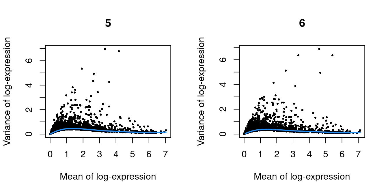
(\#fig:unref-pijuan-var-1)Per-gene variance as a function of the mean for the log-expression values in the Pijuan-Sala chimeric mouse embryo dataset. Each point represents a gene (black) with the mean-variance trend (blue) fitted to the variances.

Per-gene variance as a function of the mean for the log-expression values in the Pijuan-Sala chimeric mouse embryo dataset. Each point represents a gene (black) with the mean-variance trend (blue) fitted to the variances.

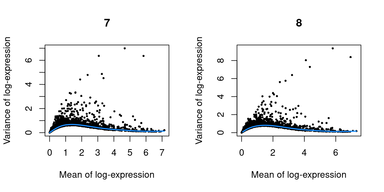
(\#fig:unref-pijuan-var-2)Per-gene variance as a function of the mean for the log-expression values in the Pijuan-Sala chimeric mouse embryo dataset. Each point represents a gene (black) with the mean-variance trend (blue) fitted to the variances.

Per-gene variance as a function of the mean for the log-expression values in the Pijuan-Sala chimeric mouse embryo dataset. Each point represents a gene (black) with the mean-variance trend (blue) fitted to the variances.

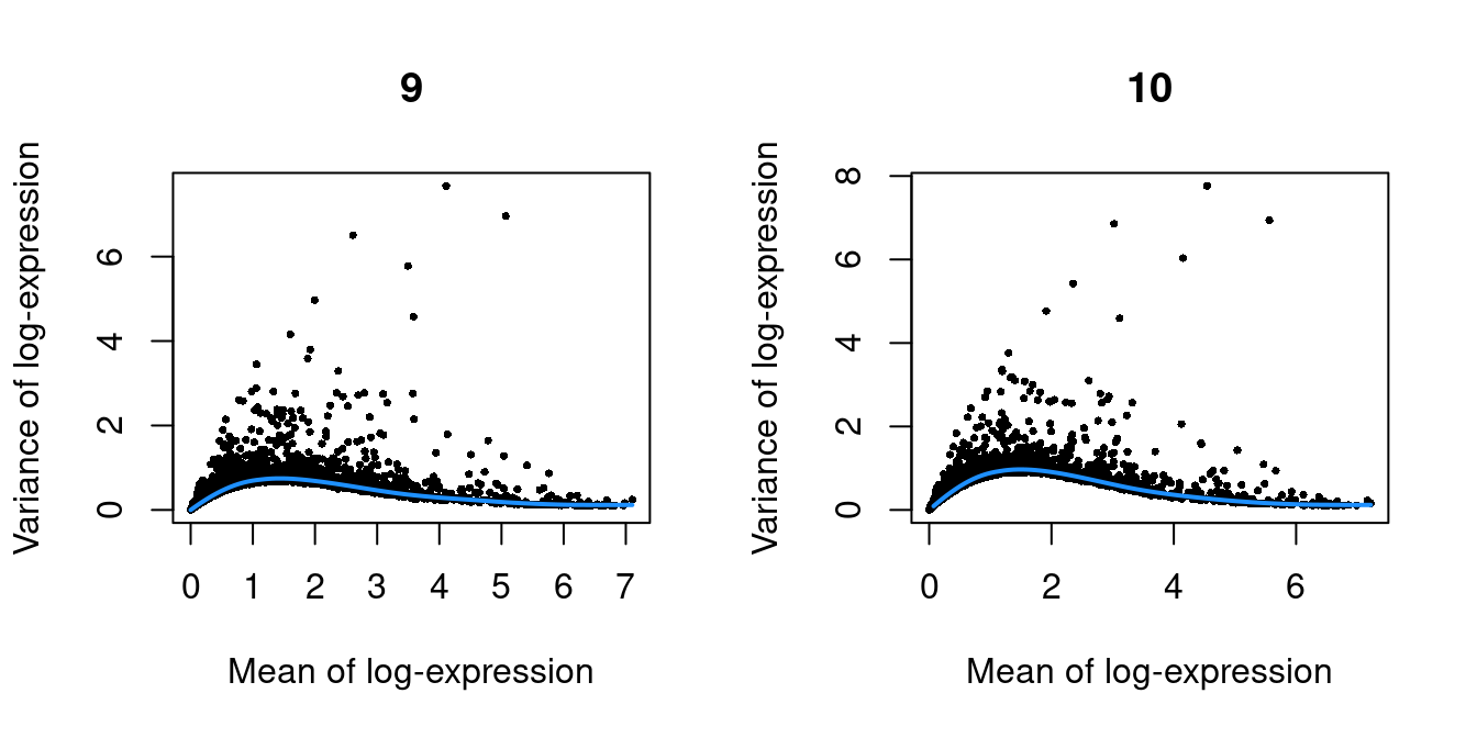
(\#fig:unref-pijuan-var-3)Per-gene variance as a function of the mean for the log-expression values in the Pijuan-Sala chimeric mouse embryo dataset. Each point represents a gene (black) with the mean-variance trend (blue) fitted to the variances.

## Merging We use a hierarchical merge to first merge together replicates with the same genotype, and then merge samples across different genotypes. ```r library(batchelor) set.seed(01001001) merged <- correctExperiments(sce.chimera, batch=sce.chimera$sample, subset.row=chosen.hvgs, PARAM=FastMnnParam( merge.order=list( list(1,3,5), # WT (3 replicates) list(2,4,6) # td-Tomato (3 replicates) ) ) ) ``` We use the percentage of variance lost as a diagnostic: ```r metadata(merged)$merge.info$lost.var ``` ``` ## 5 6 7 8 9 10 ## [1,] 0.000e+00 0.0204238 0.000e+00 0.0169321 0.000000 0.000000 ## [2,] 0.000e+00 0.0007403 0.000e+00 0.0004431 0.000000 0.015455 ## [3,] 3.089e-02 0.0000000 2.012e-02 0.0000000 0.000000 0.000000 ## [4,] 9.042e-05 0.0000000 8.298e-05 0.0000000 0.018044 0.000000 ## [5,] 4.318e-03 0.0072489 4.123e-03 0.0078254 0.003827 0.007779 ``` ## Clustering ```r g <- buildSNNGraph(merged, use.dimred="corrected") clusters <- igraph::cluster_louvain(g) colLabels(merged) <- factor(clusters$membership) ``` We examine the distribution of cells across clusters and samples. ```r table(Cluster=colLabels(merged), Sample=merged$sample) ``` ``` ## Sample ## Cluster 5 6 7 8 9 10 ## 1 86 20 62 53 151 74 ## 2 147 37 132 111 230 216 ## 3 99 16 164 128 371 275 ## 4 141 104 198 459 385 471 ## 5 96 36 291 377 171 232 ## 6 216 53 353 209 562 653 ## 7 149 73 85 85 163 377 ## 8 133 95 110 66 160 312 ## 9 82 20 74 33 165 203 ## 10 97 19 36 18 50 35 ## 11 110 41 47 38 40 147 ## 12 122 65 62 51 63 140 ## 13 157 79 131 102 133 405 ## 14 110 69 73 96 128 256 ## 15 84 47 159 351 200 620 ## 16 43 35 82 81 86 357 ## 17 165 44 208 174 200 365 ## 18 78 43 189 118 329 489 ## 19 47 22 84 50 89 128 ## 20 38 41 50 49 128 125 ## 21 1 5 0 84 0 66 ## 22 18 7 13 17 19 37 ## 23 57 29 92 78 82 190 ## 24 9 7 18 13 30 27 ## 25 11 16 20 9 47 58 ## 26 2 1 7 3 75 138 ## 27 0 2 0 51 0 5 ``` ## Dimensionality reduction We use an external algorithm to compute nearest neighbors for greater speed. ```r merged <- runTSNE(merged, dimred="corrected", external_neighbors=TRUE) merged <- runUMAP(merged, dimred="corrected", external_neighbors=TRUE) ``` ```r gridExtra::grid.arrange( plotTSNE(merged, colour_by="label", text_by="label", text_colour="red"), plotTSNE(merged, colour_by="batch") ) ```
Obligatory $t$-SNE plots of the Pijuan-Sala chimeric mouse embryo dataset, where each point represents a cell and is colored according to the assigned cluster (top) or sample of origin (bottom).

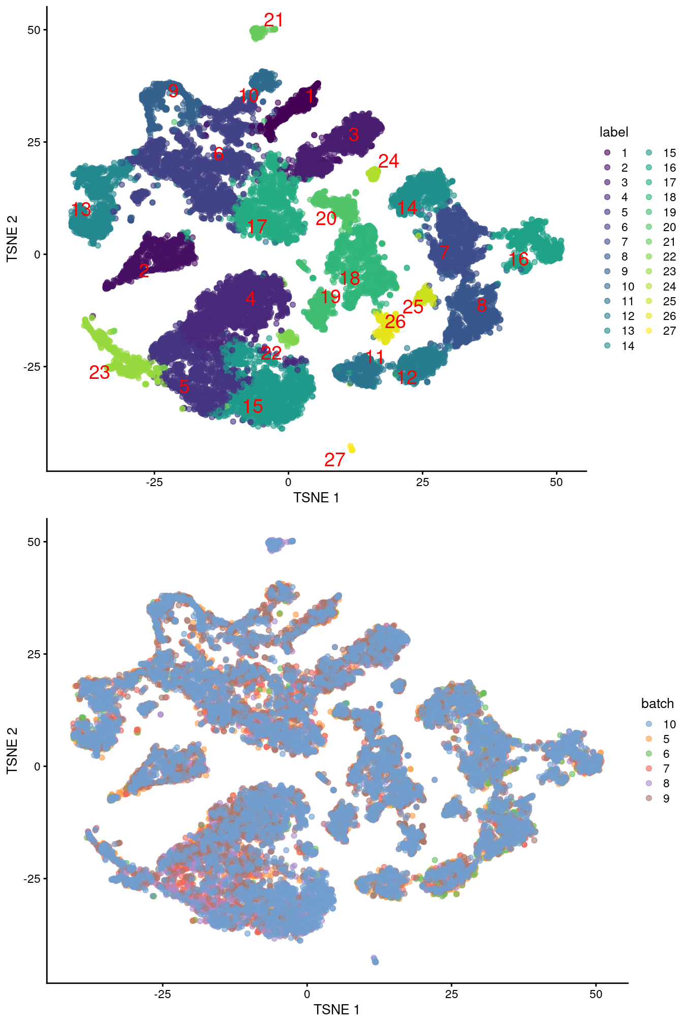
(\#fig:unref-pijuan-tsne)Obligatory $t$-SNE plots of the Pijuan-Sala chimeric mouse embryo dataset, where each point represents a cell and is colored according to the assigned cluster (top) or sample of origin (bottom).

## Session Info {-}
``` R version 4.4.0 beta (2024-04-15 r86425) Platform: x86_64-pc-linux-gnu Running under: Ubuntu 22.04.4 LTS Matrix products: default BLAS: /home/biocbuild/bbs-3.19-bioc/R/lib/libRblas.so LAPACK: /usr/lib/x86_64-linux-gnu/lapack/liblapack.so.3.10.0 locale: [1] LC_CTYPE=en_US.UTF-8 LC_NUMERIC=C [3] LC_TIME=en_GB LC_COLLATE=C [5] LC_MONETARY=en_US.UTF-8 LC_MESSAGES=en_US.UTF-8 [7] LC_PAPER=en_US.UTF-8 LC_NAME=C [9] LC_ADDRESS=C LC_TELEPHONE=C [11] LC_MEASUREMENT=en_US.UTF-8 LC_IDENTIFICATION=C time zone: America/New_York tzcode source: system (glibc) attached base packages: [1] stats4 stats graphics grDevices utils datasets methods [8] base other attached packages: [1] batchelor_1.20.0 scran_1.32.0 [3] scater_1.32.0 ggplot2_3.5.1 [5] scuttle_1.14.0 MouseGastrulationData_1.17.1 [7] SpatialExperiment_1.14.0 SingleCellExperiment_1.26.0 [9] SummarizedExperiment_1.34.0 Biobase_2.64.0 [11] GenomicRanges_1.56.0 GenomeInfoDb_1.40.0 [13] IRanges_2.38.0 S4Vectors_0.42.0 [15] BiocGenerics_0.50.0 MatrixGenerics_1.16.0 [17] matrixStats_1.3.0 BiocStyle_2.32.0 [19] rebook_1.14.0 loaded via a namespace (and not attached): [1] jsonlite_1.8.8 CodeDepends_0.6.6 [3] magrittr_2.0.3 ggbeeswarm_0.7.2 [5] magick_2.8.3 farver_2.1.1 [7] rmarkdown_2.26 zlibbioc_1.50.0 [9] vctrs_0.6.5 memoise_2.0.1 [11] DelayedMatrixStats_1.26.0 htmltools_0.5.8.1 [13] S4Arrays_1.4.0 AnnotationHub_3.12.0 [15] curl_5.2.1 BiocNeighbors_1.22.0 [17] SparseArray_1.4.0 sass_0.4.9 [19] bslib_0.7.0 cachem_1.0.8 [21] ResidualMatrix_1.14.0 igraph_2.0.3 [23] mime_0.12 lifecycle_1.0.4 [25] pkgconfig_2.0.3 rsvd_1.0.5 [27] Matrix_1.7-0 R6_2.5.1 [29] fastmap_1.1.1 GenomeInfoDbData_1.2.12 [31] digest_0.6.35 colorspace_2.1-0 [33] AnnotationDbi_1.66.0 dqrng_0.3.2 [35] irlba_2.3.5.1 ExperimentHub_2.12.0 [37] RSQLite_2.3.6 beachmat_2.20.0 [39] labeling_0.4.3 filelock_1.0.3 [41] fansi_1.0.6 httr_1.4.7 [43] abind_1.4-5 compiler_4.4.0 [45] bit64_4.0.5 withr_3.0.0 [47] BiocParallel_1.38.0 viridis_0.6.5 [49] DBI_1.2.2 highr_0.10 [51] rappdirs_0.3.3 DelayedArray_0.30.0 [53] rjson_0.2.21 bluster_1.14.0 [55] tools_4.4.0 vipor_0.4.7 [57] beeswarm_0.4.0 glue_1.7.0 [59] grid_4.4.0 Rtsne_0.17 [61] cluster_2.1.6 generics_0.1.3 [63] gtable_0.3.5 BiocSingular_1.20.0 [65] ScaledMatrix_1.12.0 metapod_1.12.0 [67] utf8_1.2.4 XVector_0.44.0 [69] ggrepel_0.9.5 BiocVersion_3.19.1 [71] pillar_1.9.0 limma_3.60.0 [73] BumpyMatrix_1.12.0 dplyr_1.1.4 [75] BiocFileCache_2.12.0 lattice_0.22-6 [77] bit_4.0.5 tidyselect_1.2.1 [79] locfit_1.5-9.9 Biostrings_2.72.0 [81] knitr_1.46 gridExtra_2.3 [83] bookdown_0.39 edgeR_4.2.0 [85] xfun_0.43 statmod_1.5.0 [87] UCSC.utils_1.0.0 yaml_2.3.8 [89] evaluate_0.23 codetools_0.2-20 [91] tibble_3.2.1 BiocManager_1.30.22 [93] graph_1.82.0 cli_3.6.2 [95] uwot_0.2.2 munsell_0.5.1 [97] jquerylib_0.1.4 Rcpp_1.0.12 [99] dir.expiry_1.12.0 dbplyr_2.5.0 [101] png_0.1-8 XML_3.99-0.16.1 [103] parallel_4.4.0 blob_1.2.4 [105] sparseMatrixStats_1.16.0 viridisLite_0.4.2 [107] scales_1.3.0 purrr_1.0.2 [109] crayon_1.5.2 rlang_1.1.3 [111] cowplot_1.1.3 KEGGREST_1.44.0 ```