---
bibliography: ref.bib
---
# Cross-annotating mouse brains
## Loading the data
We load the classic @zeisel2015brain dataset as our reference.
Here, we'll rely on the fact that the authors have already performed quality control.
```r
library(scRNAseq)
sceZ <- ZeiselBrainData()
```
We compute log-expression values for use in marker detection inside `SingleR()`.
```r
library(scater)
sceZ <- logNormCounts(sceZ)
```
We examine the distribution of labels in this reference.
```r
table(sceZ$level2class)
```
```
##
## (none) Astro1 Astro2 CA1Pyr1 CA1Pyr2 CA1PyrInt CA2Pyr2 Choroid
## 189 68 61 380 447 49 41 10
## ClauPyr Epend Int1 Int10 Int11 Int12 Int13 Int14
## 5 20 12 21 10 21 15 22
## Int15 Int16 Int2 Int3 Int4 Int5 Int6 Int7
## 18 20 24 10 15 20 22 23
## Int8 Int9 Mgl1 Mgl2 Oligo1 Oligo2 Oligo3 Oligo4
## 26 11 17 16 45 98 87 106
## Oligo5 Oligo6 Peric Pvm1 Pvm2 S1PyrDL S1PyrL23 S1PyrL4
## 125 359 21 32 33 81 74 26
## S1PyrL5 S1PyrL5a S1PyrL6 S1PyrL6b SubPyr Vend1 Vend2 Vsmc
## 16 28 39 21 22 32 105 62
```
We load the @tasic2016adult dataset as our test.
While not strictly necessary, we remove putative low-quality cells to simplify later interpretation.
```r
sceT <- TasicBrainData()
sceT <- addPerCellQC(sceT, subsets=list(mito=grep("^mt_", rownames(sceT))))
qc <- quickPerCellQC(colData(sceT),
percent_subsets=c("subsets_mito_percent", "altexps_ERCC_percent"))
sceT <- sceT[,which(!qc$discard)]
```
The Tasic dataset was generated using read-based technologies so we need to adjust for the transcript length.
```r
library(AnnotationHub)
mm.db <- AnnotationHub()[["AH73905"]]
mm.exons <- exonsBy(mm.db, by="gene")
mm.exons <- reduce(mm.exons)
mm.len <- sum(width(mm.exons))
mm.symb <- mapIds(mm.db, keys=names(mm.len), keytype="GENEID", column="SYMBOL")
names(mm.len) <- mm.symb
library(scater)
keep <- intersect(names(mm.len), rownames(sceT))
sceT <- sceT[keep,]
assay(sceT, "TPM") <- calculateTPM(sceT, lengths=mm.len[keep])
```
## Applying the annotation
We apply `SingleR()` with Wilcoxon rank sum test-based marker detection to annotate the Tasic dataset with the Zeisel labels.
```r
library(SingleR)
pred.tasic <- SingleR(test=sceT, ref=sceZ, labels=sceZ$level2class,
assay.type.test="TPM", de.method="wilcox")
```
We examine the distribution of predicted labels:
```r
table(pred.tasic$labels)
```
```
##
## Astro1 Astro2 CA1Pyr2 CA2Pyr2 ClauPyr Int1 Int10 Int11
## 1 5 1 3 1 152 98 2
## Int12 Int13 Int14 Int15 Int16 Int2 Int3 Int4
## 9 18 24 16 10 146 94 29
## Int6 Int7 Int8 Int9 Oligo1 Oligo2 Oligo3 Oligo4
## 14 2 35 31 8 1 7 1
## Oligo6 Peric S1PyrDL S1PyrL23 S1PyrL4 S1PyrL5 S1PyrL5a S1PyrL6
## 1 1 320 73 16 4 201 46
## S1PyrL6b SubPyr
## 72 5
```
We can also examine the number of discarded cells for each label:
```r
table(Label=pred.tasic$labels,
Lost=is.na(pred.tasic$pruned.labels))
```
```
## Lost
## Label FALSE TRUE
## Astro1 1 0
## Astro2 5 0
## CA1Pyr2 1 0
## CA2Pyr2 3 0
## ClauPyr 1 0
## Int1 152 0
## Int10 98 0
## Int11 2 0
## Int12 9 0
## Int13 18 0
## Int14 23 1
## Int15 16 0
## Int16 10 0
## Int2 144 2
## Int3 94 0
## Int4 29 0
## Int6 14 0
## Int7 2 0
## Int8 35 0
## Int9 31 0
## Oligo1 8 0
## Oligo2 1 0
## Oligo3 7 0
## Oligo4 1 0
## Oligo6 1 0
## Peric 1 0
## S1PyrDL 304 16
## S1PyrL23 73 0
## S1PyrL4 16 0
## S1PyrL5 4 0
## S1PyrL5a 200 1
## S1PyrL6 45 1
## S1PyrL6b 72 0
## SubPyr 5 0
```
## Diagnostics
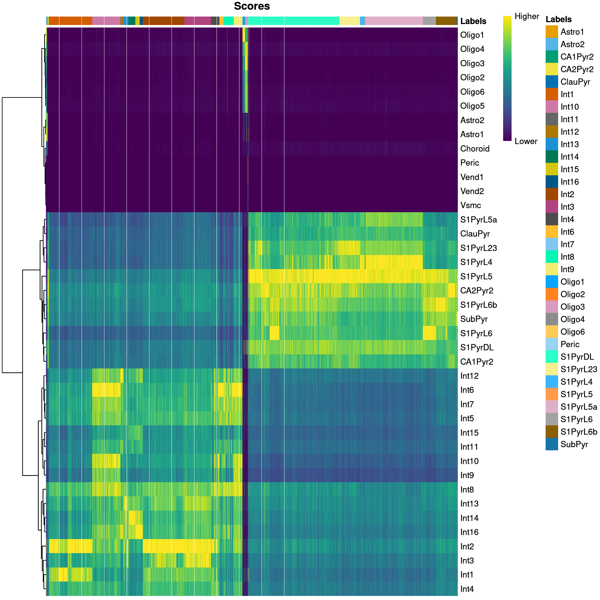
We visualize the assignment scores for each label in Figure \@ref(fig:unref-brain-score-heatmap).
```r
plotScoreHeatmap(pred.tasic)
```
(\#fig:unref-brain-score-heatmap)Heatmap of the (normalized) assignment scores for each cell (column) in the Tasic test dataset with respect to each label (row) in the Zeisel reference dataset. The final assignment for each cell is shown in the annotation bar at the top.
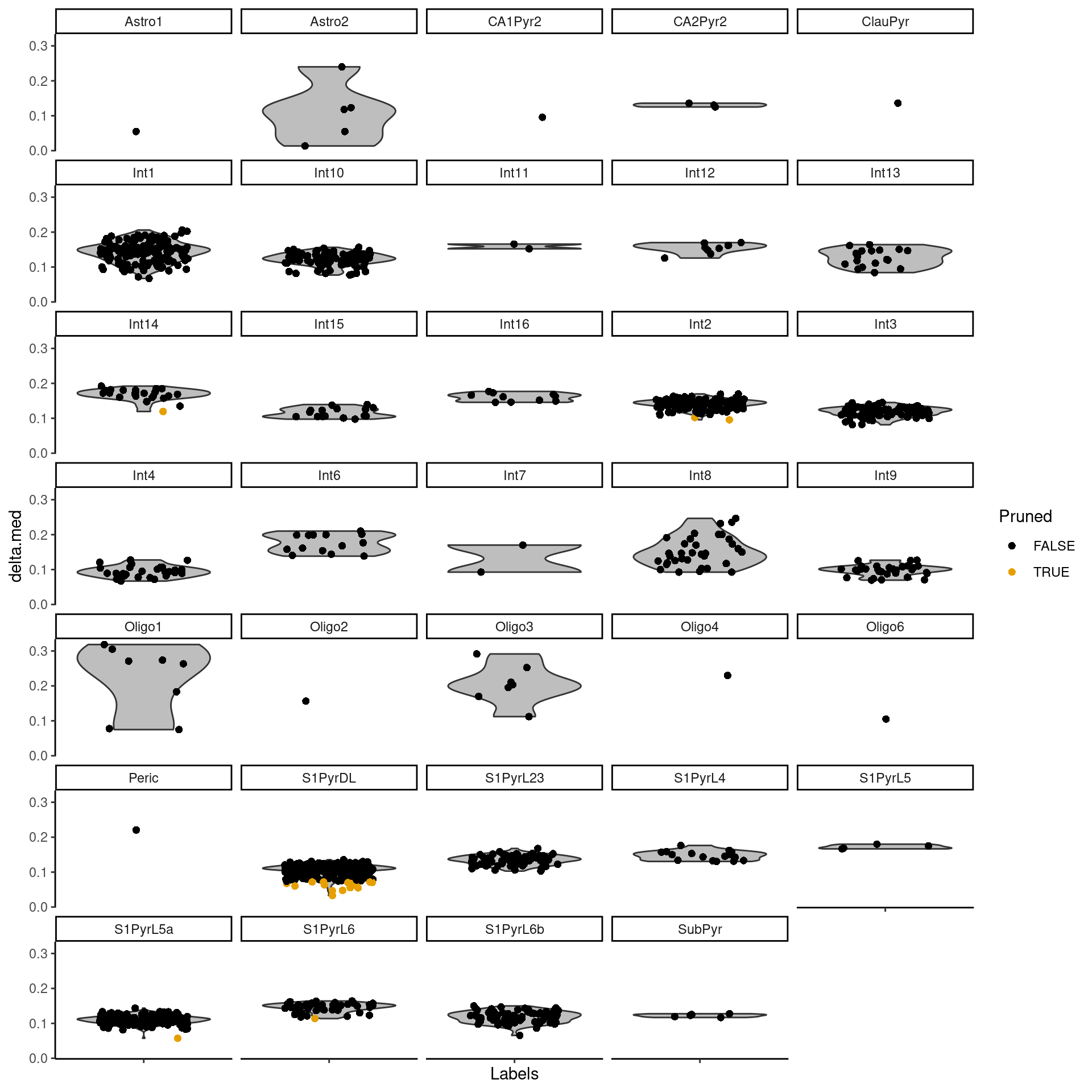
The delta for each cell is visualized in Figure \@ref(fig:unref-brain-delta-dist).
```r
plotDeltaDistribution(pred.tasic)
```
(\#fig:unref-brain-delta-dist)Distributions of the deltas for each cell in the Tasic dataset assigned to each label in the Zeisel dataset. Each cell is represented by a point; low-quality assignments that were pruned out are colored in orange.
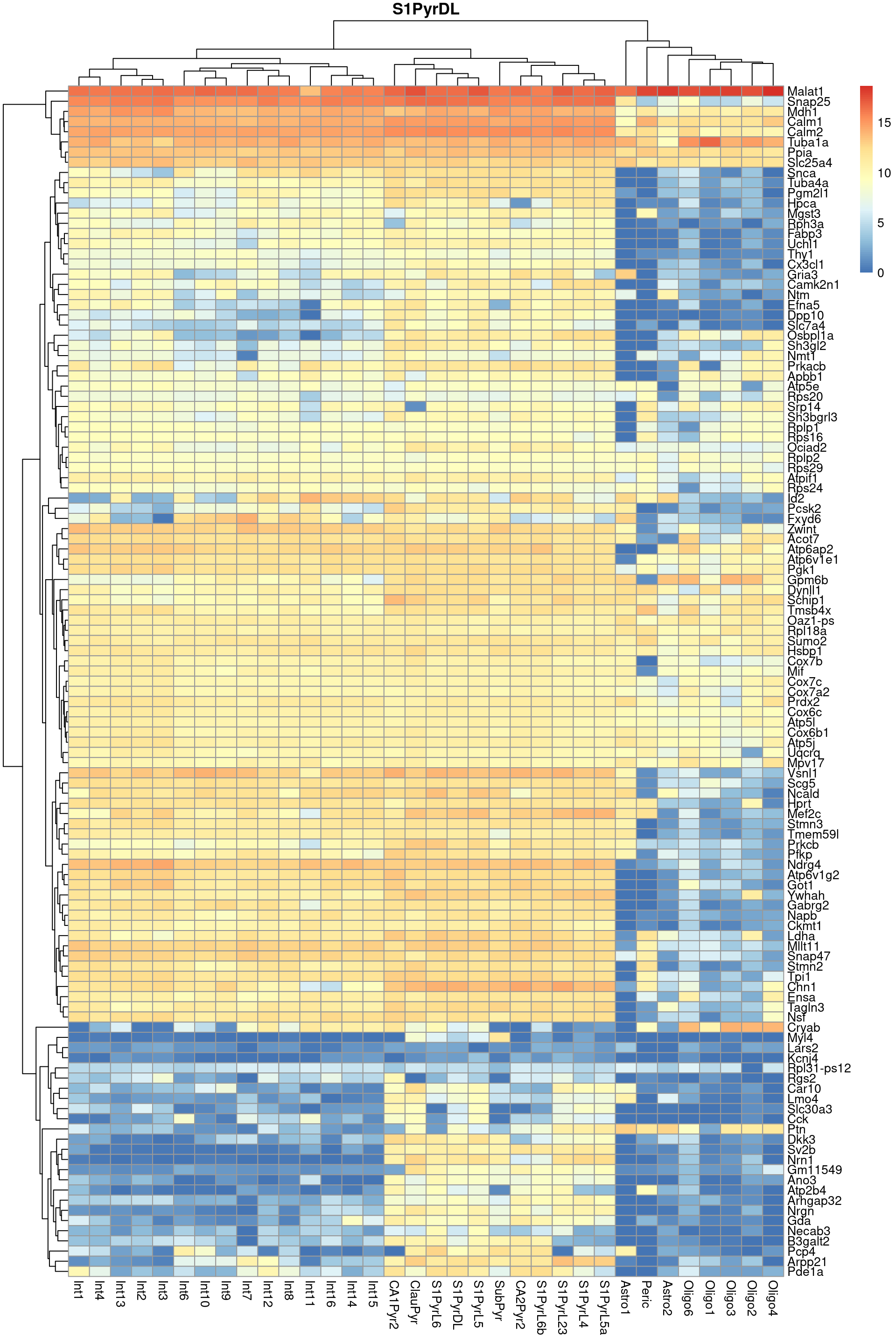
Finally, we visualize the heatmaps of the marker genes for the most frequent label in Figure \@ref(fig:unref-brain-marker-heat).
We could show these for all labels but I wouldn't want to bore you with a parade of large heatmaps.
```r
library(scater)
collected <- list()
all.markers <- metadata(pred.tasic)$de.genes
sceT <- logNormCounts(sceT)
top.label <- names(sort(table(pred.tasic$labels), decreasing=TRUE))[1]
per.label <- sumCountsAcrossCells(logcounts(sceT),
ids=pred.tasic$labels, average=TRUE)
per.label <- assay(per.label)[unique(unlist(all.markers[[top.label]])),]
pheatmap::pheatmap(per.label, main=top.label)
```
(\#fig:unref-brain-marker-heat)Heatmap of log-expression values in the Tasic dataset for all marker genes upregulated in the most frequent label from the Zeisel reference dataset.
## Comparison to clusters
For comparison, we will perform a quick unsupervised analysis of the Grun dataset.
We model the variances using the spike-in data and we perform graph-based clustering.
```r
library(scran)
decT <- modelGeneVarWithSpikes(sceT, "ERCC")
set.seed(1000100)
sceT <- denoisePCA(sceT, decT, subset.row=getTopHVGs(decT, n=2500))
library(bluster)
sceT$cluster <- clusterRows(reducedDim(sceT, "PCA"), NNGraphParam())
```
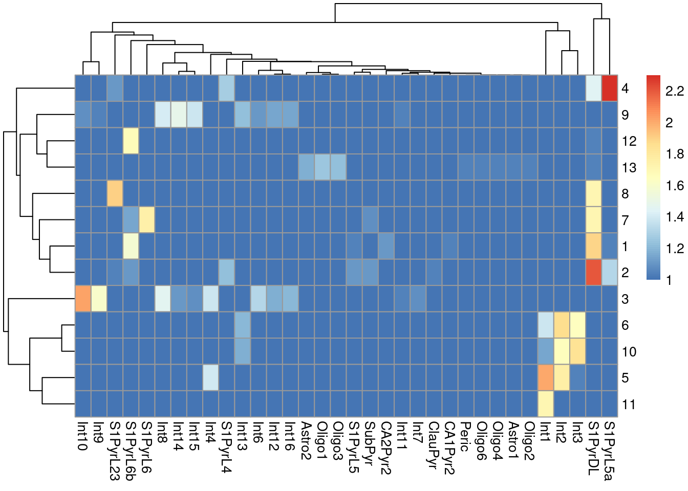
We do not observe a clean 1:1 mapping between clusters and labels in Figure \@ref(fig:unref-brain-label-clusters),
probably because many of the labels represent closely related cell types that are difficult to distinguish.
```r
tab <- table(cluster=sceT$cluster, label=pred.tasic$labels)
pheatmap::pheatmap(log10(tab+10))
```
(\#fig:unref-brain-label-clusters)Heatmap of the log-transformed number of cells in each combination of label (column) and cluster (row) in the Tasic dataset.
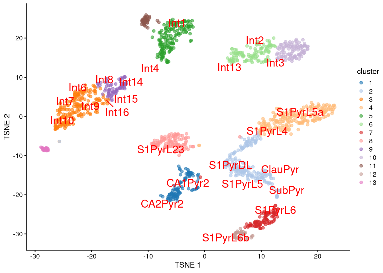
We proceed to the most important part of the analysis.
Yes, that's right, the $t$-SNE plot (Figure \@ref(fig:unref-brain-label-tsne)).
```r
set.seed(101010100)
sceT <- runTSNE(sceT, dimred="PCA")
plotTSNE(sceT, colour_by="cluster", text_colour="red",
text_by=I(pred.tasic$labels))
```
(\#fig:unref-brain-label-tsne)$t$-SNE plot of the Tasic dataset, where each point is a cell and is colored by the assigned cluster. Reference labels from the Zeisel dataset are also placed on the median coordinate across all cells assigned with that label.