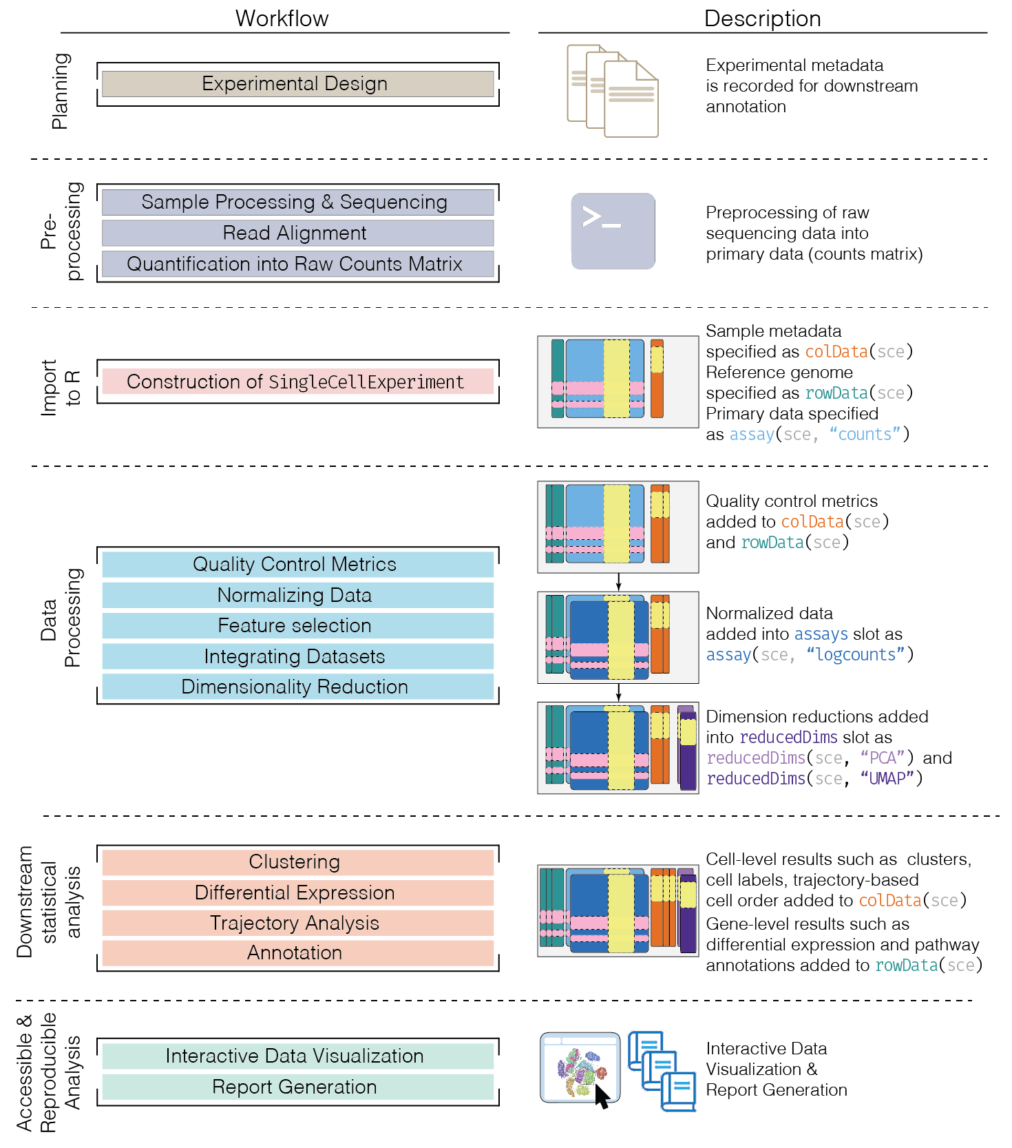
# Analysis overview
## Outline
This chapter provides an overview of the framework of a typical scRNA-seq analysis workflow (Figure \@ref(fig:scworkflow)).
(\#fig:scworkflow)Schematic of a typical scRNA-seq analysis workflow. Each stage (separated by dashed lines) consists of a number of specific steps, many of which operate on and modify a `SingleCellExperiment` instance.
In the simplest case, the workflow has the following form:
1. We compute quality control metrics to remove low-quality cells that would interfere with downstream analyses.
These cells may have been damaged during processing or may not have been fully captured by the sequencing protocol.
Common metrics includes the total counts per cell, the proportion of spike-in or mitochondrial reads and the number of detected features.
2. We convert the counts into normalized expression values to eliminate cell-specific biases (e.g., in capture efficiency).
This allows us to perform explicit comparisons across cells in downstream steps like clustering.
We also apply a transformation, typically log, to adjust for the mean-variance relationship.
3. We perform feature selection to pick a subset of interesting features for downstream analysis.
This is done by modelling the variance across cells for each gene and retaining genes that are highly variable.
The aim is to reduce computational overhead and noise from uninteresting genes.
4. We apply dimensionality reduction to compact the data and further reduce noise.
Principal components analysis is typically used to obtain an initial low-rank representation for more computational work,
followed by more aggressive methods like $t$-stochastic neighbor embedding for visualization purposes.
5. We cluster cells into groups according to similarities in their (normalized) expression profiles.
This aims to obtain groupings that serve as empirical proxies for distinct biological states.
We typically interpret these groupings by identifying differentially expressed marker genes between clusters.
Subsequent chapters will describe each analysis step in more detail.
## Quick start (simple)
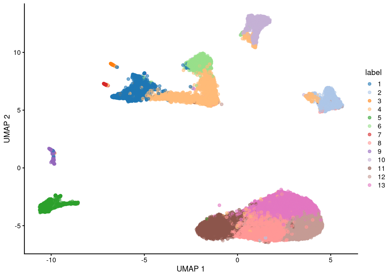
Here, we use the a droplet-based retina dataset from @macosko2015highly, provided in the *[scRNAseq](https://bioconductor.org/packages/3.18/scRNAseq)* package.
This starts from a count matrix and finishes with clusters (Figure \@ref(fig:quick-start-umap)) in preparation for biological interpretation.
Similar workflows are available in abbreviated form in later parts of the book.
```r
library(scRNAseq)
sce <- MacoskoRetinaData()
# Quality control (using mitochondrial genes).
library(scater)
is.mito <- grepl("^MT-", rownames(sce))
qcstats <- perCellQCMetrics(sce, subsets=list(Mito=is.mito))
filtered <- quickPerCellQC(qcstats, percent_subsets="subsets_Mito_percent")
sce <- sce[, !filtered$discard]
# Normalization.
sce <- logNormCounts(sce)
# Feature selection.
library(scran)
dec <- modelGeneVar(sce)
hvg <- getTopHVGs(dec, prop=0.1)
# PCA.
library(scater)
set.seed(1234)
sce <- runPCA(sce, ncomponents=25, subset_row=hvg)
# Clustering.
library(bluster)
colLabels(sce) <- clusterCells(sce, use.dimred='PCA',
BLUSPARAM=NNGraphParam(cluster.fun="louvain"))
# Visualization.
sce <- runUMAP(sce, dimred = 'PCA')
plotUMAP(sce, colour_by="label")
```
(\#fig:quick-start-umap)UMAP plot of the retina dataset, where each point is a cell and is colored by the assigned cluster identity.
```r
# Marker detection.
markers <- findMarkers(sce, test.type="wilcox", direction="up", lfc=1)
```
## Quick start (multiple batches)
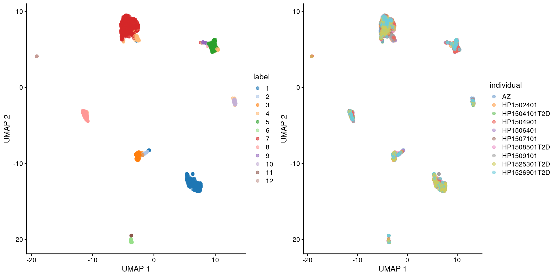
Here we use the pancreas Smart-seq2 dataset from @segerstolpe2016singlecell, again provided in the *[scRNAseq](https://bioconductor.org/packages/3.18/scRNAseq)* package.
This starts from a count matrix and finishes with clusters (Figure \@ref(fig:quick-start-umap)) with some additional tweaks to eliminate uninteresting batch effects between individuals.
Note that a more elaborate analysis of the same dataset with justifications for each step is available in [Workflow Chapter 8](http://bioconductor.org/books/3.18/OSCA.workflows/segerstolpe-human-pancreas-smart-seq2.html#segerstolpe-human-pancreas-smart-seq2).
```r
sce <- SegerstolpePancreasData()
# Quality control (using ERCCs).
qcstats <- perCellQCMetrics(sce)
filtered <- quickPerCellQC(qcstats, percent_subsets="altexps_ERCC_percent")
sce <- sce[, !filtered$discard]
# Normalization.
sce <- logNormCounts(sce)
# Feature selection, blocking on the individual of origin.
dec <- modelGeneVar(sce, block=sce$individual)
hvg <- getTopHVGs(dec, prop=0.1)
# Batch correction.
library(batchelor)
set.seed(1234)
sce <- correctExperiments(sce, batch=sce$individual,
subset.row=hvg, correct.all=TRUE)
# Clustering.
colLabels(sce) <- clusterCells(sce, use.dimred='corrected')
# Visualization.
sce <- runUMAP(sce, dimred = 'corrected')
gridExtra::grid.arrange(
plotUMAP(sce, colour_by="label"),
plotUMAP(sce, colour_by="individual"),
ncol=2
)
```
(\#fig:quick-start2-umap)UMAP plot of the pancreas dataset, where each point is a cell and is colored by the assigned cluster identity (left) or the individual of origin (right).
```r
# Marker detection, blocking on the individual of origin.
markers <- findMarkers(sce, test.type="wilcox", direction="up", lfc=1)
```
## Session Info {-}