# Human PBMC with surface proteins (10X Genomics)
## Introduction
Here, we describe a brief analysis of _yet another_ peripheral blood mononuclear cell (PBMC) dataset from 10X Genomics [@zheng2017massively].
Data are publicly available from the [10X Genomics website](https://support.10xgenomics.com/single-cell-vdj/datasets/3.0.0/vdj_v1_mm_c57bl6_pbmc_5gex), from which we download the filtered gene/barcode count matrices for gene expression and cell surface proteins.
## Data loading
```r
library(BiocFileCache)
bfc <- BiocFileCache(ask=FALSE)
exprs.data <- bfcrpath(bfc, file.path(
"http://cf.10xgenomics.com/samples/cell-vdj/3.1.0",
"vdj_v1_hs_pbmc3",
"vdj_v1_hs_pbmc3_filtered_feature_bc_matrix.tar.gz"))
untar(exprs.data, exdir=tempdir())
library(DropletUtils)
sce.pbmc <- read10xCounts(file.path(tempdir(), "filtered_feature_bc_matrix"))
sce.pbmc <- splitAltExps(sce.pbmc, rowData(sce.pbmc)$Type)
```
## Quality control
```r
unfiltered <- sce.pbmc
```
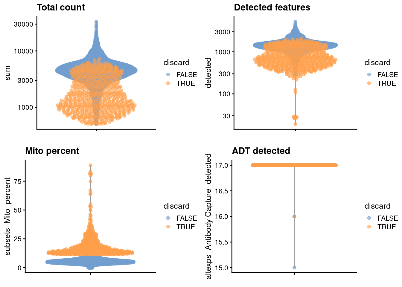
We discard cells with high mitochondrial proportions and few detectable ADT counts.
```r
library(scater)
is.mito <- grep("^MT-", rowData(sce.pbmc)$Symbol)
stats <- perCellQCMetrics(sce.pbmc, subsets=list(Mito=is.mito))
high.mito <- isOutlier(stats$subsets_Mito_percent, type="higher")
low.adt <- stats$`altexps_Antibody Capture_detected` < nrow(altExp(sce.pbmc))/2
discard <- high.mito | low.adt
sce.pbmc <- sce.pbmc[,!discard]
```
We examine some of the statistics:
```r
summary(high.mito)
```
```
## Mode FALSE TRUE
## logical 6660 571
```
```r
summary(low.adt)
```
```
## Mode FALSE
## logical 7231
```
```r
summary(discard)
```
```
## Mode FALSE TRUE
## logical 6660 571
```
We examine the distribution of each QC metric (Figure \@ref(fig:unref-pbmc-adt-qc)).
```r
colData(unfiltered) <- cbind(colData(unfiltered), stats)
unfiltered$discard <- discard
gridExtra::grid.arrange(
plotColData(unfiltered, y="sum", colour_by="discard") +
scale_y_log10() + ggtitle("Total count"),
plotColData(unfiltered, y="detected", colour_by="discard") +
scale_y_log10() + ggtitle("Detected features"),
plotColData(unfiltered, y="subsets_Mito_percent",
colour_by="discard") + ggtitle("Mito percent"),
plotColData(unfiltered, y="altexps_Antibody Capture_detected",
colour_by="discard") + ggtitle("ADT detected"),
ncol=2
)
```
(\#fig:unref-pbmc-adt-qc)Distribution of each QC metric in the PBMC dataset, where each point is a cell and is colored by whether or not it was discarded by the outlier-based QC approach.
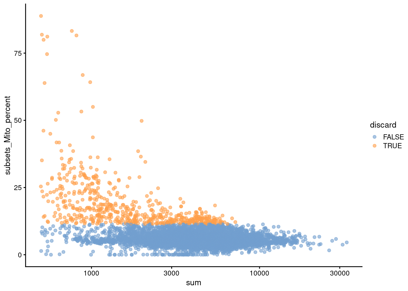
We also plot the mitochondrial proportion against the total count for each cell, as one does (Figure \@ref(fig:unref-pbmc-adt-qc-mito)).
```r
plotColData(unfiltered, x="sum", y="subsets_Mito_percent",
colour_by="discard") + scale_x_log10()
```
(\#fig:unref-pbmc-adt-qc-mito)Percentage of UMIs mapped to mitochondrial genes against the totalcount for each cell.
## Normalization
Computing size factors for the gene expression and ADT counts.
```r
library(scran)
set.seed(1000)
clusters <- quickCluster(sce.pbmc)
sce.pbmc <- computeSumFactors(sce.pbmc, cluster=clusters)
altExp(sce.pbmc) <- computeMedianFactors(altExp(sce.pbmc))
sce.pbmc <- applySCE(sce.pbmc, logNormCounts)
```
We generate some summary statistics for both sets of size factors:
```r
summary(sizeFactors(sce.pbmc))
```
```
## Min. 1st Qu. Median Mean 3rd Qu. Max.
## 0.074 0.719 0.908 1.000 1.133 8.858
```
```r
summary(sizeFactors(altExp(sce.pbmc)))
```
```
## Min. 1st Qu. Median Mean 3rd Qu. Max.
## 0.10 0.70 0.83 1.00 1.03 227.36
```
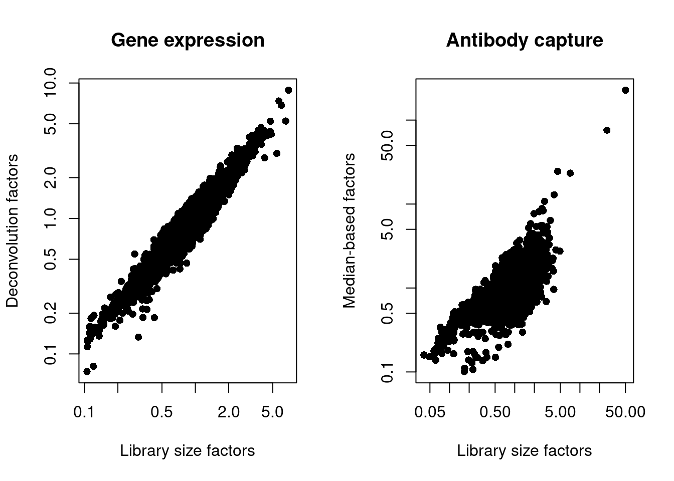
We also look at the distribution of size factors compared to the library size for each set of features (Figure \@ref(fig:unref-norm-pbmc-adt)).
```r
par(mfrow=c(1,2))
plot(librarySizeFactors(sce.pbmc), sizeFactors(sce.pbmc), pch=16,
xlab="Library size factors", ylab="Deconvolution factors",
main="Gene expression", log="xy")
plot(librarySizeFactors(altExp(sce.pbmc)), sizeFactors(altExp(sce.pbmc)), pch=16,
xlab="Library size factors", ylab="Median-based factors",
main="Antibody capture", log="xy")
```
(\#fig:unref-norm-pbmc-adt)Plot of the deconvolution size factors for the gene expression values (left) or the median-based size factors for the ADT expression values (right) compared to the library size-derived factors for the corresponding set of features. Each point represents a cell.
## Dimensionality reduction
We omit the PCA step for the ADT expression matrix, given that it is already so low-dimensional,
and progress directly to $t$-SNE and UMAP visualizations.
```r
set.seed(100000)
altExp(sce.pbmc) <- runTSNE(altExp(sce.pbmc))
set.seed(1000000)
altExp(sce.pbmc) <- runUMAP(altExp(sce.pbmc))
```
## Clustering
We perform graph-based clustering on the ADT data and use the assignments as the column labels of the alternative Experiment.
```r
g.adt <- buildSNNGraph(altExp(sce.pbmc), k=10, d=NA)
clust.adt <- igraph::cluster_walktrap(g.adt)$membership
colLabels(altExp(sce.pbmc)) <- factor(clust.adt)
```
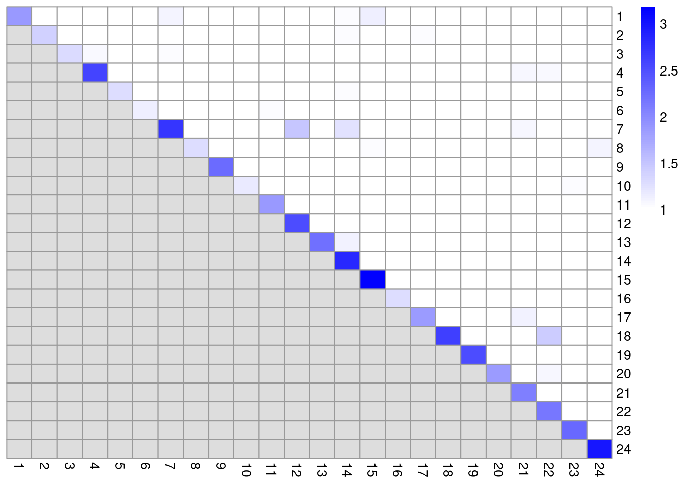
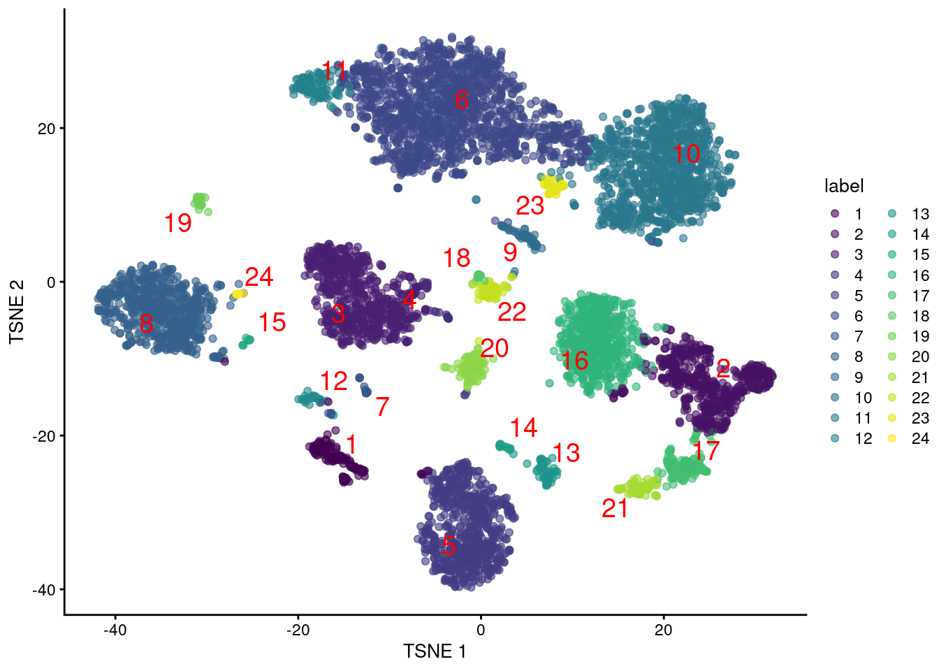
We examine some basic statistics about the size of each cluster,
their separation (Figure \@ref(fig:unref-clustmod-pbmc-adt))
and their distribution in our $t$-SNE plot (Figure \@ref(fig:unref-tsne-pbmc-adt)).
```r
table(colLabels(altExp(sce.pbmc)))
```
```
##
## 1 2 3 4 5 6 7 8 9 10 11 12 13 14 15 16
## 160 507 662 39 691 1415 32 650 76 1037 121 47 68 25 15 562
## 17 18 19 20 21 22 23 24
## 139 32 44 120 84 65 52 17
```
```r
library(bluster)
mod <- pairwiseModularity(g.adt, clust.adt, as.ratio=TRUE)
library(pheatmap)
pheatmap::pheatmap(log10(mod + 10), cluster_row=FALSE, cluster_col=FALSE,
color=colorRampPalette(c("white", "blue"))(101))
```
(\#fig:unref-clustmod-pbmc-adt)Heatmap of the pairwise cluster modularity scores in the PBMC dataset, computed based on the shared nearest neighbor graph derived from the ADT expression values.
(\#fig:unref-tsne-pbmc-adt)Obligatory $t$-SNE plot of PBMC dataset based on its ADT expression values, where each point is a cell and is colored by the cluster of origin. Cluster labels are also overlaid at the median coordinates across all cells in the cluster.