# Lawlor human pancreas (SMARTer)

<script>
document.addEventListener("click", function (event) {
    if (event.target.classList.contains("rebook-collapse")) {
        event.target.classList.toggle("active");
        var content = event.target.nextElementSibling;
        if (content.style.display === "block") {
            content.style.display = "none";
        } else {
            content.style.display = "block";
        }
    }
})
</script>

<style>
.rebook-collapse {
  background-color: #eee;
  color: #444;
  cursor: pointer;
  padding: 18px;
  width: 100%;
  border: none;
  text-align: left;
  outline: none;
  font-size: 15px;
}

.rebook-content {
  padding: 0 18px;
  display: none;
  overflow: hidden;
  background-color: #f1f1f1;
}
</style>

## Introduction

This performs an analysis of the @lawlor2017singlecell dataset,
consisting of human pancreas cells from various donors.

## Data loading


```r
library(scRNAseq)
sce.lawlor <- LawlorPancreasData()
```


```r
library(AnnotationHub)
edb <- AnnotationHub()[["AH73881"]]
anno <- select(edb, keys=rownames(sce.lawlor), keytype="GENEID", 
    columns=c("SYMBOL", "SEQNAME"))
rowData(sce.lawlor) <- anno[match(rownames(sce.lawlor), anno[,1]),-1]
```

## Quality control


```r
unfiltered <- sce.lawlor
```


```r
library(scater)
stats <- perCellQCMetrics(sce.lawlor, 
    subsets=list(Mito=which(rowData(sce.lawlor)$SEQNAME=="MT")))
qc <- quickPerCellQC(stats, percent_subsets="subsets_Mito_percent",
    batch=sce.lawlor$`islet unos id`)
sce.lawlor <- sce.lawlor[,!qc$discard]
```


```r
colData(unfiltered) <- cbind(colData(unfiltered), stats)
unfiltered$discard <- qc$discard

gridExtra::grid.arrange(
    plotColData(unfiltered, x="islet unos id", y="sum", colour_by="discard") +
        scale_y_log10() + ggtitle("Total count") +
        theme(axis.text.x = element_text(angle = 90)),
    plotColData(unfiltered, x="islet unos id", y="detected", 
        colour_by="discard") + scale_y_log10() + ggtitle("Detected features") +
        theme(axis.text.x = element_text(angle = 90)), 
    plotColData(unfiltered, x="islet unos id", y="subsets_Mito_percent",
        colour_by="discard") + ggtitle("Mito percent") +
        theme(axis.text.x = element_text(angle = 90)),
    ncol=2
)
```

<div class="figure">
<img src="lawlor-pancreas_files/figure-html/unref-lawlor-qc-dist-1.png" alt="Distribution of each QC metric across cells from each donor of the Lawlor pancreas dataset. Each point represents a cell and is colored according to whether that cell was discarded." width="960" />
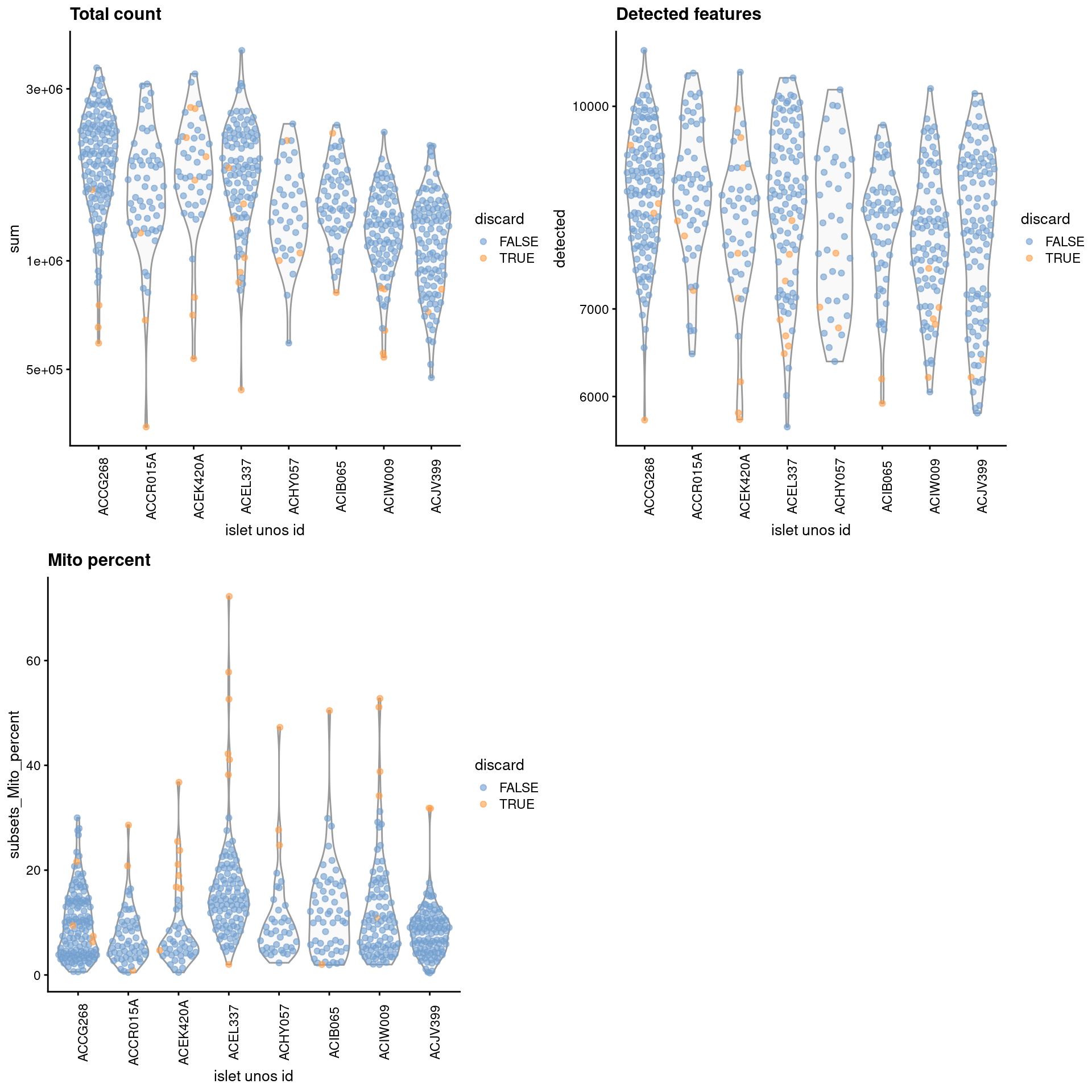
<p class="caption">(\#fig:unref-lawlor-qc-dist)Distribution of each QC metric across cells from each donor of the Lawlor pancreas dataset. Each point represents a cell and is colored according to whether that cell was discarded.</p>
</div>


```r
plotColData(unfiltered, x="sum", y="subsets_Mito_percent",
    colour_by="discard") + scale_x_log10()
```

<div class="figure">
<img src="lawlor-pancreas_files/figure-html/unref-lawlor-qc-comp-1.png" alt="Percentage of mitochondrial reads in each cell in the 416B dataset compared to the total count. Each point represents a cell and is colored according to whether that cell was discarded." width="672" />
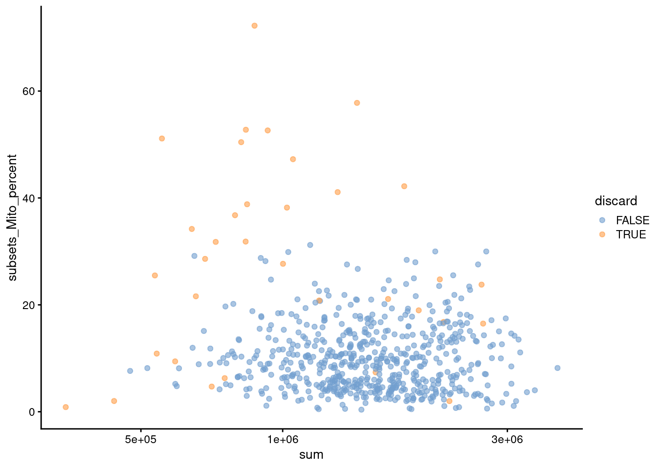
<p class="caption">(\#fig:unref-lawlor-qc-comp)Percentage of mitochondrial reads in each cell in the 416B dataset compared to the total count. Each point represents a cell and is colored according to whether that cell was discarded.</p>
</div>


```r
colSums(as.matrix(qc))
```

```
##              low_lib_size            low_n_features high_subsets_Mito_percent 
##                         9                         5                        25 
##                   discard 
##                        34
```

## Normalization


```r
library(scran)
set.seed(1000)
clusters <- quickCluster(sce.lawlor)
sce.lawlor <- computeSumFactors(sce.lawlor, clusters=clusters)
sce.lawlor <- logNormCounts(sce.lawlor)
```


```r
summary(sizeFactors(sce.lawlor))
```

```
##    Min. 1st Qu.  Median    Mean 3rd Qu.    Max. 
##   0.295   0.781   0.963   1.000   1.182   2.629
```


```r
plot(librarySizeFactors(sce.lawlor), sizeFactors(sce.lawlor), pch=16,
    xlab="Library size factors", ylab="Deconvolution factors", log="xy")
```

<div class="figure">
<img src="lawlor-pancreas_files/figure-html/unref-lawlor-norm-1.png" alt="Relationship between the library size factors and the deconvolution size factors in the Lawlor pancreas dataset." width="672" />
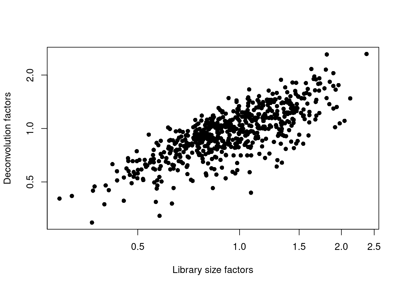
<p class="caption">(\#fig:unref-lawlor-norm)Relationship between the library size factors and the deconvolution size factors in the Lawlor pancreas dataset.</p>
</div>

## Variance modelling

Using age as a proxy for the donor.


```r
dec.lawlor <- modelGeneVar(sce.lawlor, block=sce.lawlor$`islet unos id`)
chosen.genes <- getTopHVGs(dec.lawlor, n=2000)
```


```r
par(mfrow=c(4,2))
blocked.stats <- dec.lawlor$per.block
for (i in colnames(blocked.stats)) {
    current <- blocked.stats[[i]]
    plot(current$mean, current$total, main=i, pch=16, cex=0.5,
        xlab="Mean of log-expression", ylab="Variance of log-expression")
    curfit <- metadata(current)
    curve(curfit$trend(x), col='dodgerblue', add=TRUE, lwd=2)
}
```

<div class="figure">
<img src="lawlor-pancreas_files/figure-html/unnamed-chunk-4-1.png" alt="Per-gene variance as a function of the mean for the log-expression values in the Lawlor pancreas dataset. Each point represents a gene (black) with the mean-variance trend (blue) fitted separately for each donor." width="672" />
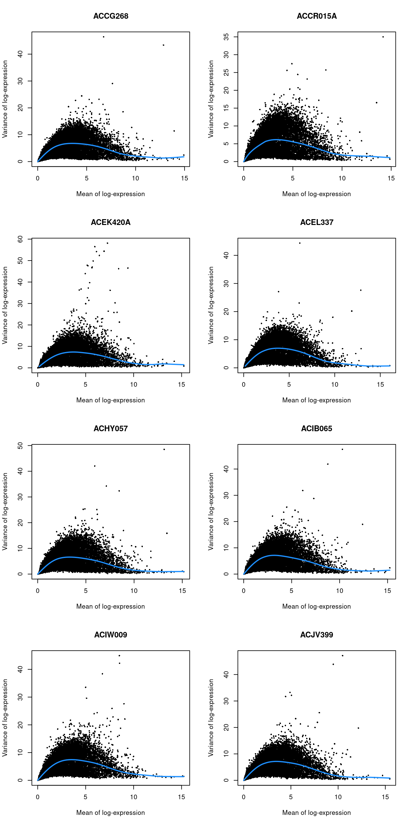
<p class="caption">(\#fig:unnamed-chunk-4)Per-gene variance as a function of the mean for the log-expression values in the Lawlor pancreas dataset. Each point represents a gene (black) with the mean-variance trend (blue) fitted separately for each donor.</p>
</div>

## Dimensionality reduction


```r
library(BiocSingular)
set.seed(101011001)
sce.lawlor <- runPCA(sce.lawlor, subset_row=chosen.genes, ncomponents=25)
sce.lawlor <- runTSNE(sce.lawlor, dimred="PCA")
```

## Clustering


```r
snn.gr <- buildSNNGraph(sce.lawlor, use.dimred="PCA")
colLabels(sce.lawlor) <- factor(igraph::cluster_walktrap(snn.gr)$membership)
```


```r
table(colLabels(sce.lawlor), sce.lawlor$`cell type`)
```

```
##    
##     Acinar Alpha Beta Delta Ductal Gamma/PP None/Other Stellate
##   1      1     0    0    13      2       16          2        0
##   2      0     1   76     1      0        0          0        0
##   3      0   161    1     0      0        1          2        0
##   4      0     1    0     1      0        0          5       19
##   5      0     0  175     4      1        0          1        0
##   6     22     0    0     0      0        0          0        0
##   7      0    75    0     0      0        0          0        0
##   8      0     0    0     1     20        0          2        0
```


```r
table(colLabels(sce.lawlor), sce.lawlor$`islet unos id`)
```

```
##    
##     ACCG268 ACCR015A ACEK420A ACEL337 ACHY057 ACIB065 ACIW009 ACJV399
##   1       8        2        2       4       4       4       9       1
##   2      14        3        2      33       3       2       4      17
##   3      36       23       14      13      14      14      21      30
##   4       7        1        0       1       0       4       9       4
##   5      34       10        4      39       7      23      24      40
##   6       0        2       13       0       0       0       5       2
##   7      32       12        0       5       6       7       4       9
##   8       1        1        2       1       2       1      12       3
```


```r
gridExtra::grid.arrange(
    plotTSNE(sce.lawlor, colour_by="label"),
    plotTSNE(sce.lawlor, colour_by="islet unos id"),
    ncol=2
)
```

<div class="figure">
<img src="lawlor-pancreas_files/figure-html/unref-grun-tsne-1.png" alt="Obligatory $t$-SNE plots of the Lawlor pancreas dataset. Each point represents a cell that is colored by cluster (left) or batch (right)." width="672" />
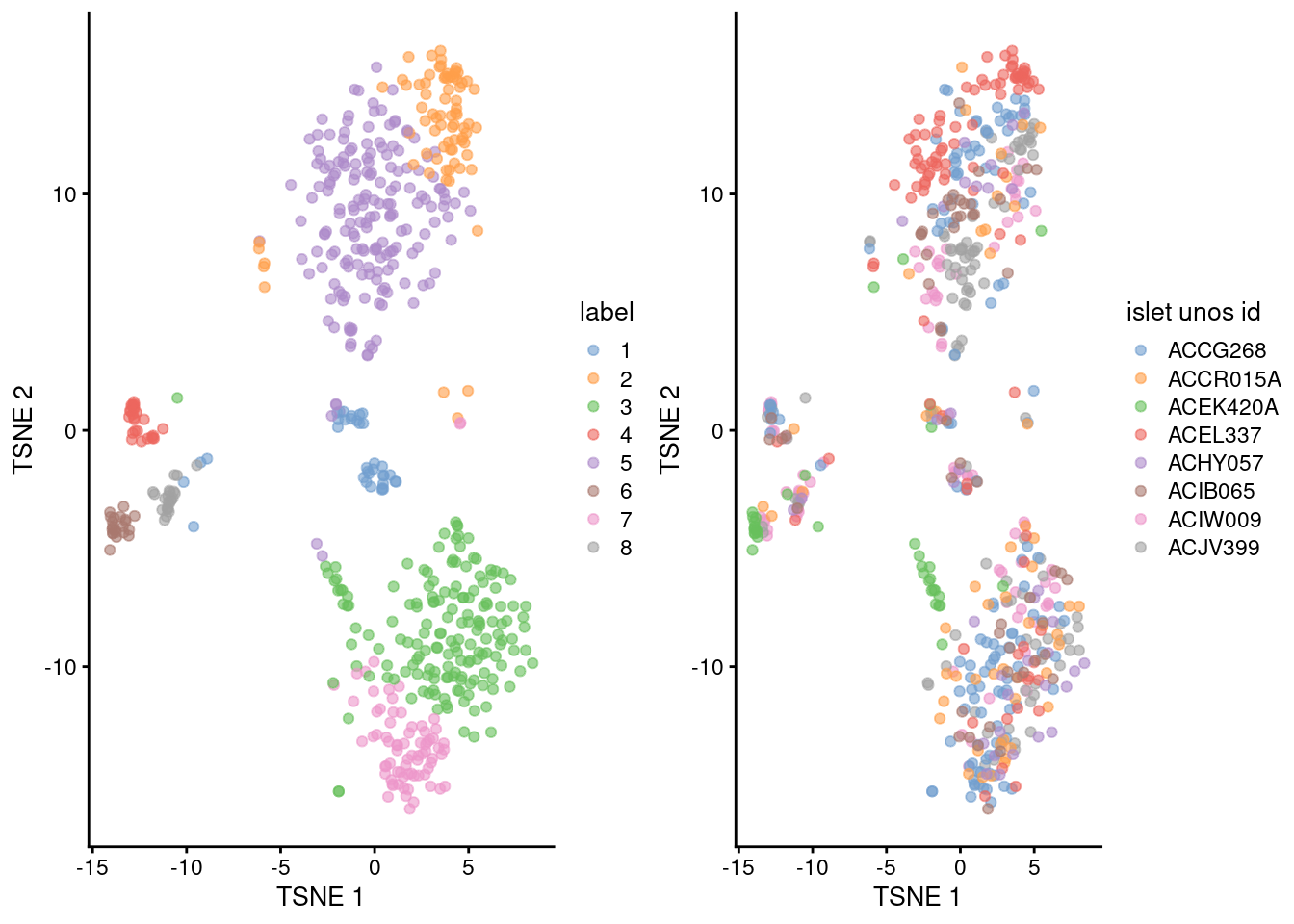
<p class="caption">(\#fig:unref-grun-tsne)Obligatory $t$-SNE plots of the Lawlor pancreas dataset. Each point represents a cell that is colored by cluster (left) or batch (right).</p>
</div>

## Session Info {-}

<button class="rebook-collapse">View session info</button>
<div class="rebook-content">
```
R version 4.2.1 (2022-06-23)
Platform: x86_64-pc-linux-gnu (64-bit)
Running under: Ubuntu 20.04.5 LTS

Matrix products: default
BLAS:   /home/biocbuild/bbs-3.16-bioc/R/lib/libRblas.so
LAPACK: /home/biocbuild/bbs-3.16-bioc/R/lib/libRlapack.so

locale:
 [1] LC_CTYPE=en_US.UTF-8       LC_NUMERIC=C              
 [3] LC_TIME=en_GB              LC_COLLATE=C              
 [5] LC_MONETARY=en_US.UTF-8    LC_MESSAGES=en_US.UTF-8   
 [7] LC_PAPER=en_US.UTF-8       LC_NAME=C                 
 [9] LC_ADDRESS=C               LC_TELEPHONE=C            
[11] LC_MEASUREMENT=en_US.UTF-8 LC_IDENTIFICATION=C       

attached base packages:
[1] stats4    stats     graphics  grDevices utils     datasets  methods  
[8] base     

other attached packages:
 [1] BiocSingular_1.14.0         scran_1.26.0               
 [3] scater_1.26.0               ggplot2_3.3.6              
 [5] scuttle_1.8.0               ensembldb_2.22.0           
 [7] AnnotationFilter_1.22.0     GenomicFeatures_1.50.0     
 [9] AnnotationDbi_1.60.0        AnnotationHub_3.6.0        
[11] BiocFileCache_2.6.0         dbplyr_2.2.1               
[13] scRNAseq_2.11.0             SingleCellExperiment_1.20.0
[15] SummarizedExperiment_1.28.0 Biobase_2.58.0             
[17] GenomicRanges_1.50.0        GenomeInfoDb_1.34.0        
[19] IRanges_2.32.0              S4Vectors_0.36.0           
[21] BiocGenerics_0.44.0         MatrixGenerics_1.10.0      
[23] matrixStats_0.62.0          BiocStyle_2.26.0           
[25] rebook_1.8.0               

loaded via a namespace (and not attached):
  [1] igraph_1.3.5                  lazyeval_0.2.2               
  [3] BiocParallel_1.32.0           digest_0.6.30                
  [5] htmltools_0.5.3               viridis_0.6.2                
  [7] fansi_1.0.3                   magrittr_2.0.3               
  [9] memoise_2.0.1                 ScaledMatrix_1.6.0           
 [11] cluster_2.1.4                 limma_3.54.0                 
 [13] Biostrings_2.66.0             prettyunits_1.1.1            
 [15] colorspace_2.0-3              blob_1.2.3                   
 [17] rappdirs_0.3.3                ggrepel_0.9.1                
 [19] xfun_0.34                     dplyr_1.0.10                 
 [21] crayon_1.5.2                  RCurl_1.98-1.9               
 [23] jsonlite_1.8.3                graph_1.76.0                 
 [25] glue_1.6.2                    gtable_0.3.1                 
 [27] zlibbioc_1.44.0               XVector_0.38.0               
 [29] DelayedArray_0.24.0           scales_1.2.1                 
 [31] edgeR_3.40.0                  DBI_1.1.3                    
 [33] Rcpp_1.0.9                    viridisLite_0.4.1            
 [35] xtable_1.8-4                  progress_1.2.2               
 [37] dqrng_0.3.0                   bit_4.0.4                    
 [39] rsvd_1.0.5                    metapod_1.6.0                
 [41] httr_1.4.4                    dir.expiry_1.6.0             
 [43] ellipsis_0.3.2                pkgconfig_2.0.3              
 [45] XML_3.99-0.12                 farver_2.1.1                 
 [47] CodeDepends_0.6.5             sass_0.4.2                   
 [49] locfit_1.5-9.6                utf8_1.2.2                   
 [51] labeling_0.4.2                tidyselect_1.2.0             
 [53] rlang_1.0.6                   later_1.3.0                  
 [55] munsell_0.5.0                 BiocVersion_3.16.0           
 [57] tools_4.2.1                   cachem_1.0.6                 
 [59] cli_3.4.1                     generics_0.1.3               
 [61] RSQLite_2.2.18                ExperimentHub_2.6.0          
 [63] evaluate_0.17                 stringr_1.4.1                
 [65] fastmap_1.1.0                 yaml_2.3.6                   
 [67] knitr_1.40                    bit64_4.0.5                  
 [69] purrr_0.3.5                   KEGGREST_1.38.0              
 [71] sparseMatrixStats_1.10.0      mime_0.12                    
 [73] xml2_1.3.3                    biomaRt_2.54.0               
 [75] compiler_4.2.1                beeswarm_0.4.0               
 [77] filelock_1.0.2                curl_4.3.3                   
 [79] png_0.1-7                     interactiveDisplayBase_1.36.0
 [81] statmod_1.4.37                tibble_3.1.8                 
 [83] bslib_0.4.0                   stringi_1.7.8                
 [85] highr_0.9                     bluster_1.8.0                
 [87] lattice_0.20-45               ProtGenerics_1.30.0          
 [89] Matrix_1.5-1                  vctrs_0.5.0                  
 [91] pillar_1.8.1                  lifecycle_1.0.3              
 [93] BiocManager_1.30.19           jquerylib_0.1.4              
 [95] BiocNeighbors_1.16.0          cowplot_1.1.1                
 [97] bitops_1.0-7                  irlba_2.3.5.1                
 [99] httpuv_1.6.6                  rtracklayer_1.58.0           
[101] R6_2.5.1                      BiocIO_1.8.0                 
[103] bookdown_0.29                 promises_1.2.0.1             
[105] gridExtra_2.3                 vipor_0.4.5                  
[107] codetools_0.2-18              assertthat_0.2.1             
[109] rjson_0.2.21                  withr_2.5.0                  
[111] GenomicAlignments_1.34.0      Rsamtools_2.14.0             
[113] GenomeInfoDbData_1.2.9        parallel_4.2.1               
[115] hms_1.1.2                     grid_4.2.1                   
[117] beachmat_2.14.0               rmarkdown_2.17               
[119] DelayedMatrixStats_1.20.0     Rtsne_0.16                   
[121] shiny_1.7.3                   ggbeeswarm_0.6.0             
[123] restfulr_0.0.15              
```
</div>