---
bibliography: ref.bib
---
# H3K27me3, wild-type versus knock-out
## Overview
Here, we perform a window-based DB analysis to identify regions of differential H3K27me3 enrichment in mouse lung epithelium.
H3K27me3 is associated with transcriptional repression and is usually observed with broad regions of enrichment.
The aim of this workflow is to demonstrate how to analyze these broad marks with *[csaw](https://bioconductor.org/packages/3.13/csaw)*,
especially at variable resolutions with multiple window sizes.
We use H3K27me3 ChIP-seq data from a study comparing wild-type (WT) and _Ezh2_ knock-out (KO) animals [@galvis2015repression],
contains two biological replicates for each genotype.
We download BAM files and indices using *[chipseqDBData](https://bioconductor.org/packages/3.13/chipseqDBData)*.
```r
library(chipseqDBData)
h3k27me3data <- H3K27me3Data()
h3k27me3data
```
```
## DataFrame with 4 rows and 3 columns
## Name Description Path
##
## 1 SRR1274188 control H3K27me3 (1)
## 2 SRR1274189 control H3K27me3 (2)
## 3 SRR1274190 Ezh2 knock-out H3K27..
## 4 SRR1274191 Ezh2 knock-out H3K27..
```
## Pre-processing checks
We check some mapping statistics with *[Rsamtools](https://bioconductor.org/packages/3.13/Rsamtools)*.
```r
library(Rsamtools)
diagnostics <- list()
for (b in seq_along(h3k27me3data$Path)) {
bam <- h3k27me3data$Path[[b]]
total <- countBam(bam)$records
mapped <- countBam(bam, param=ScanBamParam(
flag=scanBamFlag(isUnmapped=FALSE)))$records
marked <- countBam(bam, param=ScanBamParam(
flag=scanBamFlag(isUnmapped=FALSE, isDuplicate=TRUE)))$records
diagnostics[[b]] <- c(Total=total, Mapped=mapped, Marked=marked)
}
diag.stats <- data.frame(do.call(rbind, diagnostics))
rownames(diag.stats) <- h3k27me3data$Name
diag.stats$Prop.mapped <- diag.stats$Mapped/diag.stats$Total*100
diag.stats$Prop.marked <- diag.stats$Marked/diag.stats$Mapped*100
diag.stats
```
```
## Total Mapped Marked Prop.mapped Prop.marked
## SRR1274188 24445704 18605240 2769679 76.11 14.89
## SRR1274189 21978677 17014171 2069203 77.41 12.16
## SRR1274190 26910067 18606352 4361393 69.14 23.44
## SRR1274191 21354963 14092438 4392541 65.99 31.17
```
We construct a `readParam` object to standardize the parameter settings in this analysis.
For consistency with the original analysis by @galvis2015repression,
we will define the blacklist using the predicted repeats from the RepeatMasker software.
```r
library(BiocFileCache)
bfc <- BiocFileCache("local", ask=FALSE)
black.path <- bfcrpath(bfc, file.path("http://hgdownload.cse.ucsc.edu",
"goldenPath/mm10/bigZips/chromOut.tar.gz"))
tmpdir <- tempfile()
dir.create(tmpdir)
untar(black.path, exdir=tmpdir)
# Iterate through all chromosomes.
collected <- list()
for (x in list.files(tmpdir, full=TRUE)) {
f <- list.files(x, full=TRUE, pattern=".fa.out")
to.get <- vector("list", 15)
to.get[[5]] <- "character"
to.get[6:7] <- "integer"
collected[[length(collected)+1]] <- read.table(f, skip=3,
stringsAsFactors=FALSE, colClasses=to.get)
}
collected <- do.call(rbind, collected)
blacklist <- GRanges(collected[,1], IRanges(collected[,2], collected[,3]))
blacklist
```
```
## GRanges object with 5147737 ranges and 0 metadata columns:
## seqnames ranges strand
##
## [1] chr1 3000001-3002128 *
## [2] chr1 3003153-3003994 *
## [3] chr1 3003994-3004054 *
## [4] chr1 3004041-3004206 *
## [5] chr1 3004207-3004270 *
## ... ... ... ...
## [5147733] chrY_JH584303_random 152557-155890 *
## [5147734] chrY_JH584303_random 155891-156883 *
## [5147735] chrY_JH584303_random 157070-157145 *
## [5147736] chrY_JH584303_random 157909-157960 *
## [5147737] chrY_JH584303_random 157953-158099 *
## -------
## seqinfo: 66 sequences from an unspecified genome; no seqlengths
```
We set the minimum mapping quality score to 10 to remove poorly or non-uniquely aligned reads.
We also restrict ourselves to the standard chromosomes.
```r
library(csaw)
param <- readParam(minq=10, discard=blacklist,
restrict=paste0("chr", c(1:19, "X", "Y")))
param
```
```
## Extracting reads in single-end mode
## Duplicate removal is turned off
## Minimum allowed mapping score is 10
## Reads are extracted from both strands
## Read extraction is limited to 21 sequences
## Reads in 5147737 regions will be discarded
```
## Counting reads into windows
Reads are then counted into sliding windows using *[csaw](https://bioconductor.org/packages/3.13/csaw)* [@lun2016csaw].
At this stage, we use a large 2 kbp window to reflect the fact that H3K27me3 exhibits broad enrichment.
This allows us to increase the size of the counts and thus detection power,
without having to be concerned about loss of genomic resolution to detect sharp binding events.
```r
win.data <- windowCounts(h3k27me3data$Path, param=param, width=2000,
spacing=500, ext=200)
win.data
```
```
## class: RangedSummarizedExperiment
## dim: 4611513 4
## metadata(6): spacing width ... param final.ext
## assays(1): counts
## rownames: NULL
## rowData names(0):
## colnames: NULL
## colData names(4): bam.files totals ext rlen
```
We use `spacing=500` to avoid redundant work when sliding a large window across the genome.
The default spacing of 50 bp would result in many windows with over 90% overlap in their positions,
increasing the amount of computational work without a meaningful improvement in resolution.
We also set the fragment length to 200 bp based on experimental knowledge of the size selection procedure.
Unlike the previous analyses, the fragment length cannot easily estimated here due to weak strand bimodality of diffuse marks.
## Filtering of low-abundance windows
We estimate the global background and remove low-abundance windows that are not enriched above this background level.
To retain a window, we require it to have at least 2-fold more coverage than the average background.
This is less stringent than the thresholds used in previous analyses, owing the weaker enrichment observed for diffuse marks.
```r
bins <- windowCounts(h3k27me3data$Path, bin=TRUE, width=10000, param=param)
filter.stat <- filterWindowsGlobal(win.data, bins)
min.fc <- 2
```
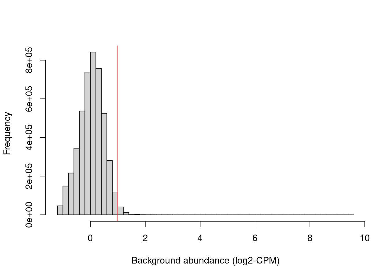
Figure \@ref(fig:h3k27me3-bghistplot) shows that chosen threshold is greater than the abundances of most bins in the genome,
presumably those corresponding to background regions.
This suggests that the filter will remove most windows lying within background regions.
```r
hist(filter.stat$filter, main="", breaks=50,
xlab="Background abundance (log2-CPM)")
abline(v=log2(min.fc), col="red")
```
(\#fig:h3k27me3-bghistplot)Histogram of average abundances across all 10 kbp genomic bins. The filter threshold is shown as the red line.
We filter out the majority of windows in background regions upon applying a modest fold-change threshold.
This leaves a small set of relevant windows for further analysis.
```r
keep <- filter.stat$filter > log2(min.fc)
summary(keep)
```
```
## Mode FALSE TRUE
## logical 4553052 58461
```
```r
filtered.data <- win.data[keep,]
```
## Normalization for composition biases
As in the CBP example, we normalize for composition biases resulting from imbalanced DB between conditions.
This is because we expect systematic DB in one direction as Ezh2 function (and thus some H3K27me3 deposition activity) is lost in the KO genotype.
```r
win.data <- normFactors(bins, se.out=win.data)
(normfacs <- win.data$norm.factors)
```
```
## [1] 0.9966 0.9969 1.0079 0.9986
```
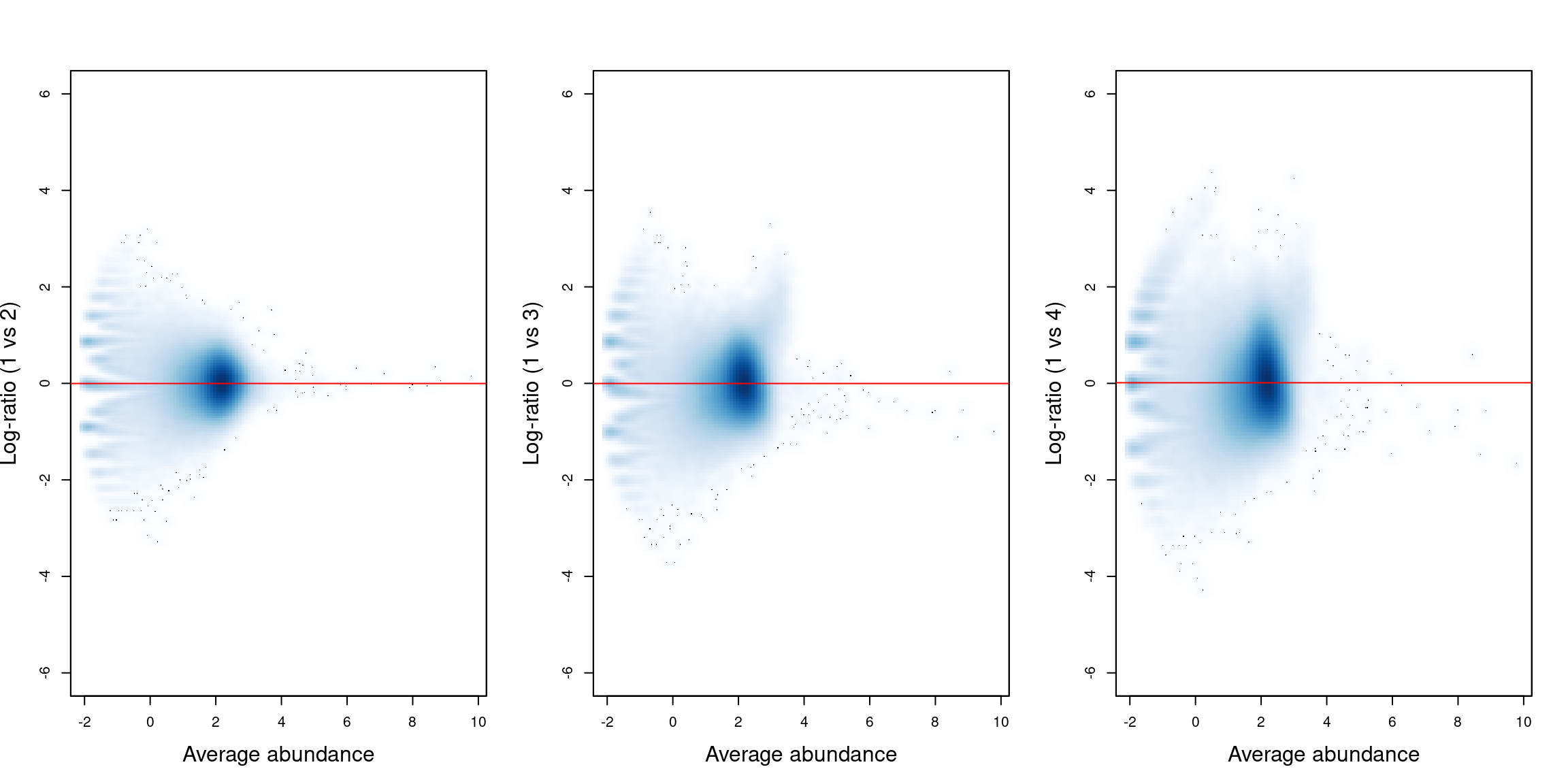
Figure \@ref(fig:h3k27me3-compoplot) shows the effect of normalization on the relative enrichment between pairs of samples.
We see that log-ratio of normalization factors passes through the centre of the cloud of background regions in each plot,
indicating that the bias has been successfully identified and removed.
```r
bin.ab <- scaledAverage(bins)
adjc <- calculateCPM(bins, use.norm.factors=FALSE)
par(cex.lab=1.5, mfrow=c(1,3))
smoothScatter(bin.ab, adjc[,1]-adjc[,2], ylim=c(-6, 6),
xlab="Average abundance", ylab="Log-ratio (1 vs 2)")
abline(h=log2(normfacs[1]/normfacs[4]), col="red")
smoothScatter(bin.ab, adjc[,1]-adjc[,3], ylim=c(-6, 6),
xlab="Average abundance", ylab="Log-ratio (1 vs 3)")
abline(h=log2(normfacs[2]/normfacs[4]), col="red")
smoothScatter(bin.ab, adjc[,1]-adjc[,4], ylim=c(-6, 6),
xlab="Average abundance", ylab="Log-ratio (1 vs 4)")
abline(h=log2(normfacs[3]/normfacs[4]), col="red")
```
(\#fig:h3k27me3-compoplot)Mean-difference plots for the bin counts, comparing sample 1 to all other samples. The red line represents the log-ratio of the normalization factors between samples.
## Statistical modelling
We first convert our `RangedSummarizedExperiment` object into a `DGEList` for modelling with *[edgeR](https://bioconductor.org/packages/3.13/edgeR)*.
```r
library(edgeR)
y <- asDGEList(filtered.data)
str(y)
```
```
## Formal class 'DGEList' [package "edgeR"] with 1 slot
## ..@ .Data:List of 2
## .. ..$ : int [1:58461, 1:4] 17 19 32 33 30 31 31 36 33 29 ...
## .. .. ..- attr(*, "dimnames")=List of 2
## .. .. .. ..$ : chr [1:58461] "1" "2" "3" "4" ...
## .. .. .. ..$ : chr [1:4] "Sample1" "Sample2" "Sample3" "Sample4"
## .. ..$ :'data.frame': 4 obs. of 3 variables:
## .. .. ..$ group : Factor w/ 1 level "1": 1 1 1 1
## .. .. ..$ lib.size : int [1:4] 10577670 9948013 8579597 5642350
## .. .. ..$ norm.factors: num [1:4] 1 1 1 1
## ..$ names: chr [1:2] "counts" "samples"
```
We then construct a design matrix for our experimental design.
Here, we use a simple one-way layout with two groups of two replicates.
```r
genotype <- h3k27me3data$Description
genotype[grep("control", genotype)] <- "wt"
genotype[grep("knock-out", genotype)] <- "ko"
genotype <- factor(genotype)
design <- model.matrix(~0+genotype)
colnames(design) <- levels(genotype)
design
```
```
## ko wt
## 1 0 1
## 2 0 1
## 3 1 0
## 4 1 0
## attr(,"assign")
## [1] 1 1
## attr(,"contrasts")
## attr(,"contrasts")$genotype
## [1] "contr.treatment"
```
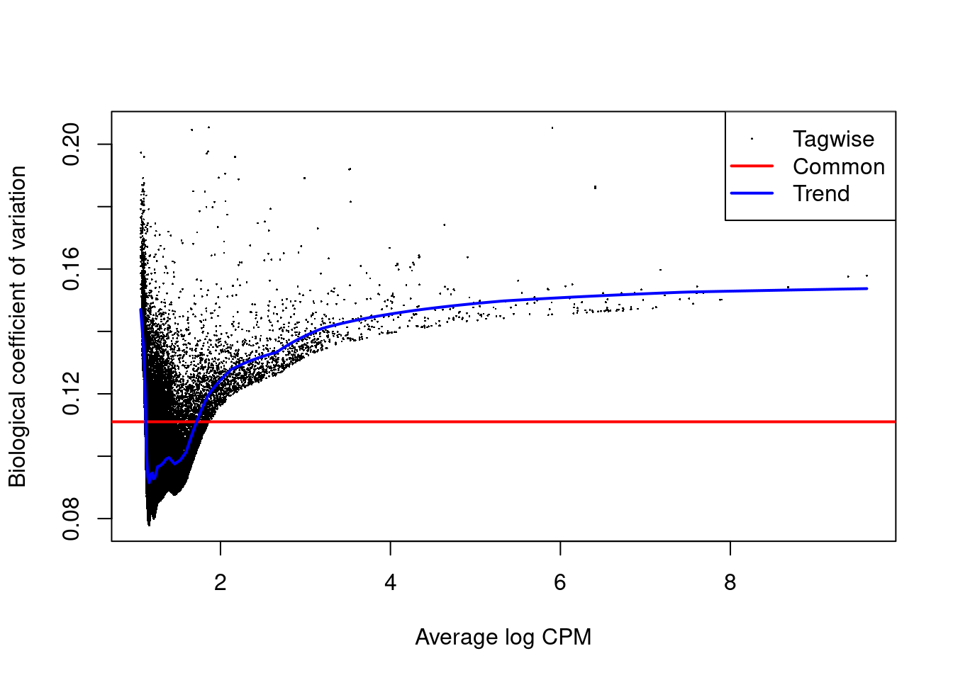
We estimate the negative binomial (NB) and quasi-likelihood (QL) dispersions for each window.
We again observe an increasing trend in the NB dispersions with respect to abundance (Figure \@ref(fig:h3k27me3-bcvplot)).
```r
y <- estimateDisp(y, design)
summary(y$trended.dispersion)
```
```
## Min. 1st Qu. Median Mean 3rd Qu. Max.
## 0.00837 0.00884 0.00942 0.01026 0.00988 0.02363
```
```r
plotBCV(y)
```
(\#fig:h3k27me3-bcvplot)Abundance-dependent trend in the BCV for each window, represented by the blue line. Common (red) and tagwise estimates (black) are also shown.
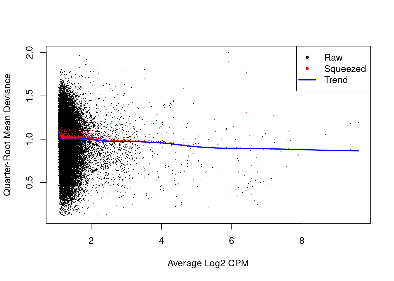
The QL dispersions are strongly shrunk towards the trend (Figure \@ref(fig:h3k27me3-qlplot)),
indicating that there is little variability in the dispersions across windows.
```r
fit <- glmQLFit(y, design, robust=TRUE)
summary(fit$df.prior)
```
```
## Min. 1st Qu. Median Mean 3rd Qu. Max.
## 0.52 90.42 90.42 90.34 90.42 90.42
```
```r
plotQLDisp(fit)
```
(\#fig:h3k27me3-qlplot)Effect of EB shrinkage on the raw QL dispersion estimate for each window (black) towards the abundance-dependent trend (blue) to obtain squeezed estimates (red).
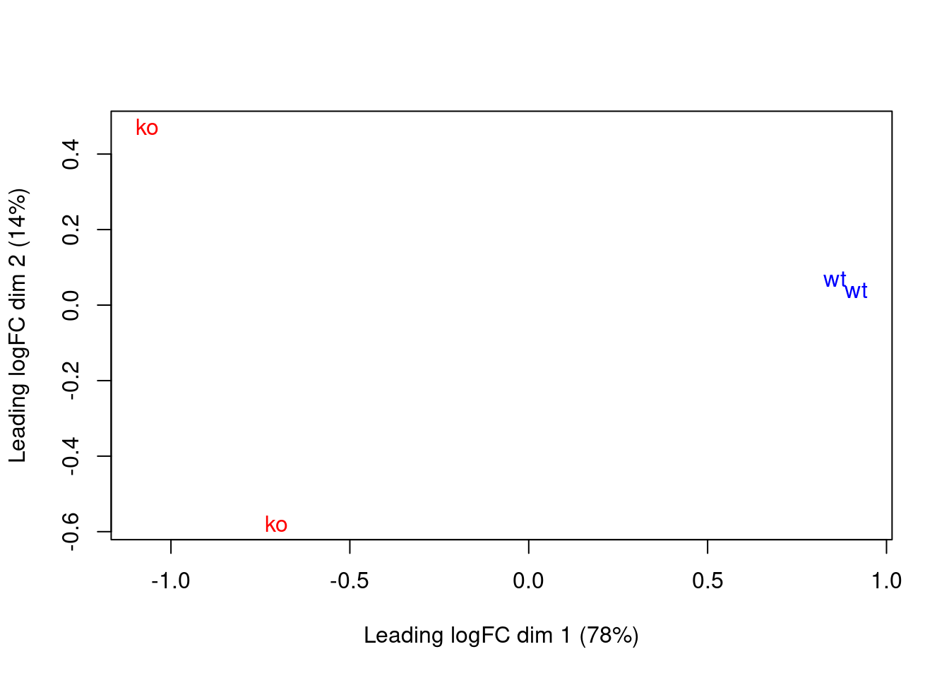
These results are consistent with the presence of systematic differences in enrichment between replicates, as discussed in Section \@ref(sec:cbp-statistical-modelling).
Nonetheless, the samples separate by genotype in the MDS plot (Figure \@ref(fig:h3k27me3-mdsplot)),
which suggests that the downstream analysis will be able to detect DB regions.
```r
plotMDS(cpm(y, log=TRUE), top=10000, labels=genotype,
col=c("red", "blue")[as.integer(genotype)])
```
(\#fig:h3k27me3-mdsplot)MDS plot with two dimensions for all samples in the H3K27me3 data set. Samples are labelled and coloured according to the genotype. A larger top set of windows was used to improve the visualization of the genome-wide differences between the WT samples.
We then test for DB between conditions in each window using the QL F-test.
```r
contrast <- makeContrasts(wt-ko, levels=design)
res <- glmQLFTest(fit, contrast=contrast)
```
## Consolidating results from multiple window sizes
Consolidation allows the analyst to incorporate information from a range of different window sizes,
each of which has a different trade-off between resolution and count size.
This is particularly useful for broad marks where the width of an enriched region can be variable,
as can the width of the differentially bound interval of an enriched region.
To demonstrate, we repeat the entire analysis using 500 bp windows.
Compared to our previous 2 kbp analysis, this provides greater spatial resolution at the cost of lowering the counts.
```r
# Counting into 500 bp windows.
win.data2 <- windowCounts(h3k27me3data$Path, param=param, width=500,
spacing=100, ext=200)
# Re-using the same normalization factors.
win.data2$norm.factors <- win.data$norm.factors
# Filtering on abundance.
filter.stat2 <- filterWindowsGlobal(win.data2, bins)
keep2 <- filter.stat2$filter > log2(min.fc)
filtered.data2 <- win.data2[keep2,]
# Performing the statistical analysis.
y2 <- asDGEList(filtered.data2)
y2 <- estimateDisp(y2, design)
fit2 <- glmQLFit(y2, design, robust=TRUE)
res2 <- glmQLFTest(fit2, contrast=contrast)
```
We consolidate the 500 bp analysis with our previous 2 kbp analysis using the `mergeWindowsList()` function.
This clusters both sets of windows together into a single set of regions.
To limit chaining effects, each region cannot be more than 30 kbp in size.
```r
merged <- mergeResultsList(list(filtered.data, filtered.data2),
tab.list=list(res$table, res2$table),
equiweight=TRUE, tol=100, merge.args=list(max.width=30000))
merged$regions
```
```
## GRanges object with 80139 ranges and 0 metadata columns:
## seqnames ranges strand
##
## [1] chr1 3050001-3052500 *
## [2] chr1 3086401-3087200 *
## [3] chr1 3098001-3098800 *
## [4] chr1 3139501-3140100 *
## [5] chr1 3211501-3212600 *
## ... ... ... ...
## [80135] chrY 90766001-90769500 *
## [80136] chrY 90774801-90775900 *
## [80137] chrY 90788501-90789000 *
## [80138] chrY 90793101-90793700 *
## [80139] chrY 90797001-90814000 *
## -------
## seqinfo: 21 sequences from an unspecified genome
```
We compute combined $p$-values using Simes' method for region-level FDR control [@simes1986; @lun2014].
This is done after weighting the contributions from the two sets of windows
to ensure that the combined $p$-value for each region is not dominated by the analysis with more (smaller) windows.
```r
tabcom <- merged$combined
is.sig <- tabcom$FDR <= 0.05
summary(is.sig)
```
```
## Mode FALSE TRUE
## logical 73136 7003
```
Ezh2 is one of the proteins responsible for depositing H3K27me3,
so we might expect that most DB regions have increased enrichment in the WT condition.
However, the opposite seems to be true here, which is an interesting result that may warrant further investigation.
```r
table(tabcom$direction[is.sig])
```
```
##
## down up
## 4803 2200
```
We also obtain statistics for the window with the lowest $p$-value in each region.
The signs of the log-fold changes are largely consistent with the `direction` numbers above.
```r
tabbest <- merged$best
is.sig.pos <- (tabbest$rep.logFC > 0)[is.sig]
summary(is.sig.pos)
```
```
## Mode FALSE TRUE
## logical 4803 2200
```
Finally, we save these results to file for future reference.
```r
out.ranges <- merged$regions
mcols(out.ranges) <- data.frame(tabcom, best.logFC=tabbest$rep.logFC)
saveRDS(file="h3k27me3_results.rds", out.ranges)
```
## Annotation and visualization
We add annotation for each region using the `detailRanges()` function,
as [previously described](https://bioconductor.org/packages/3.13/chipseqDB/vignettes/h3k9ac.html#using-the-detailranges-function).
```r
library(TxDb.Mmusculus.UCSC.mm10.knownGene)
library(org.Mm.eg.db)
anno <- detailRanges(out.ranges, orgdb=org.Mm.eg.db,
txdb=TxDb.Mmusculus.UCSC.mm10.knownGene)
mcols(out.ranges) <- cbind(mcols(out.ranges), anno)
```
We visualize one of the DB regions overlapping the _Cdx2_ gene to reproduce the results in @holik2015transcriptome.
```r
cdx2 <- genes(TxDb.Mmusculus.UCSC.mm10.knownGene)["12591"] # Cdx2 Entrez ID
cur.region <- subsetByOverlaps(out.ranges, cdx2)[1]
cur.region
```
```
## GRanges object with 1 range and 12 metadata columns:
## seqnames ranges strand | num.tests num.up.logFC
## |
## [1] chr5 147299501-147322500 * | 138 92
## num.down.logFC PValue FDR direction rep.test rep.logFC
##
## [1] 0 8.20439e-07 0.000172118 up 44791 2.95226
## best.logFC overlap left right
##
## [1] 2.60436 Cdx2:-:PE,Urad:-:PE
## -------
## seqinfo: 21 sequences from an unspecified genome
```
We use *[Gviz](https://bioconductor.org/packages/3.13/Gviz)* [@hahne2016visualizing] to plot the results.
As in the H3K9ac analysis, we set up some tracks to display genome coordinates and gene annotation.
```r
library(Gviz)
gax <- GenomeAxisTrack(col="black", fontsize=15, size=2)
greg <- GeneRegionTrack(TxDb.Mmusculus.UCSC.mm10.knownGene, showId=TRUE,
geneSymbol=TRUE, name="", background.title="transparent")
symbols <- unlist(mapIds(org.Mm.eg.db, gene(greg), "SYMBOL",
"ENTREZID", multiVals = "first"))
symbol(greg) <- symbols[gene(greg)]
```
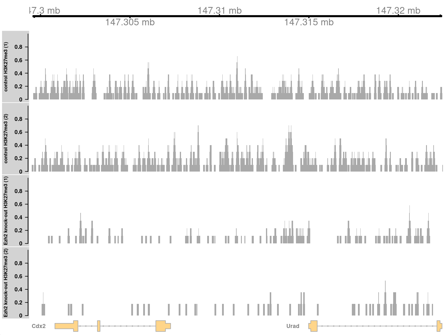
In Figure \@ref(fig:h3k27me3-tfplot), we see enrichment of H3K27me3 in the WT condition at the _Cdx2_ locus.
This is consistent with the known regulatory relationship between Ezh2 and _Cdx2_.
```r
collected <- list()
lib.sizes <- filtered.data$totals/1e6
for (i in seq_along(h3k27me3data$Path)) {
reads <- extractReads(bam.file=h3k27me3data$Path[[i]], cur.region, param=param)
cov <- as(coverage(reads)/lib.sizes[i], "GRanges")
collected[[i]] <- DataTrack(cov, type="histogram", lwd=0, ylim=c(0,1),
name=h3k27me3data$Description[i], col.axis="black", col.title="black",
fill="darkgray", col.histogram=NA)
}
plotTracks(c(gax, collected, greg), chromosome=as.character(seqnames(cur.region)),
from=start(cur.region), to=end(cur.region))
```
(\#fig:h3k27me3-tfplot)Coverage tracks for a region with H3K27me3 enrichment in KO (top two tracks) against the WT (last two tracks).
In contrast, if we look at a constitutively expressed gene, such as _Col1a2_, we find little evidence of H3K27me3 deposition.
Only a single window is retained after filtering on abundance,
and this window shows no evidence of changes in H3K27me3 enrichment between WT and KO samples.
```r
col1a2 <- genes(TxDb.Mmusculus.UCSC.mm10.knownGene)["12843"] # Col1a2 Entrez ID
cur.region <- subsetByOverlaps(out.ranges, col1a2)
cur.region
```
```
## GRanges object with 1 range and 12 metadata columns:
## seqnames ranges strand | num.tests num.up.logFC num.down.logFC
## |
## [1] chr6 4511701-4512200 * | 1 0 0
## PValue FDR direction rep.test rep.logFC best.logFC
##
## [1] 0.220691 0.432977 down 312358 -0.714484 -0.714484
## overlap left right
##
## [1] Col1a2:+:I Col1a2:+:907 Col1a2:+:161
## -------
## seqinfo: 21 sequences from an unspecified genome
```
## Session information {-}