# Segerstolpe human pancreas (Smart-seq2)
## Introduction
This performs an analysis of the @segerstolpe2016singlecell dataset,
consisting of human pancreas cells from various donors.
## Data loading
```r
library(scRNAseq)
sce.seger <- SegerstolpePancreasData()
```
```r
library(AnnotationHub)
edb <- AnnotationHub()[["AH73881"]]
symbols <- rowData(sce.seger)$symbol
ens.id <- mapIds(edb, keys=symbols, keytype="SYMBOL", column="GENEID")
ens.id <- ifelse(is.na(ens.id), symbols, ens.id)
# Removing duplicated rows.
keep <- !duplicated(ens.id)
sce.seger <- sce.seger[keep,]
rownames(sce.seger) <- ens.id[keep]
```
We simplify the names of some of the relevant column metadata fields for ease of access.
Some editing of the cell type labels is necessary for consistency with other data sets.
```r
emtab.meta <- colData(sce.seger)[,c("cell type", "disease",
"individual", "single cell well quality")]
colnames(emtab.meta) <- c("CellType", "Disease", "Donor", "Quality")
colData(sce.seger) <- emtab.meta
sce.seger$CellType <- gsub(" cell", "", sce.seger$CellType)
sce.seger$CellType <- paste0(
toupper(substr(sce.seger$CellType, 1, 1)),
substring(sce.seger$CellType, 2))
```
## Quality control
```r
unfiltered <- sce.seger
```
We remove low quality cells that were marked by the authors.
We then perform additional quality control as some of the remaining cells still have very low counts and numbers of detected features.
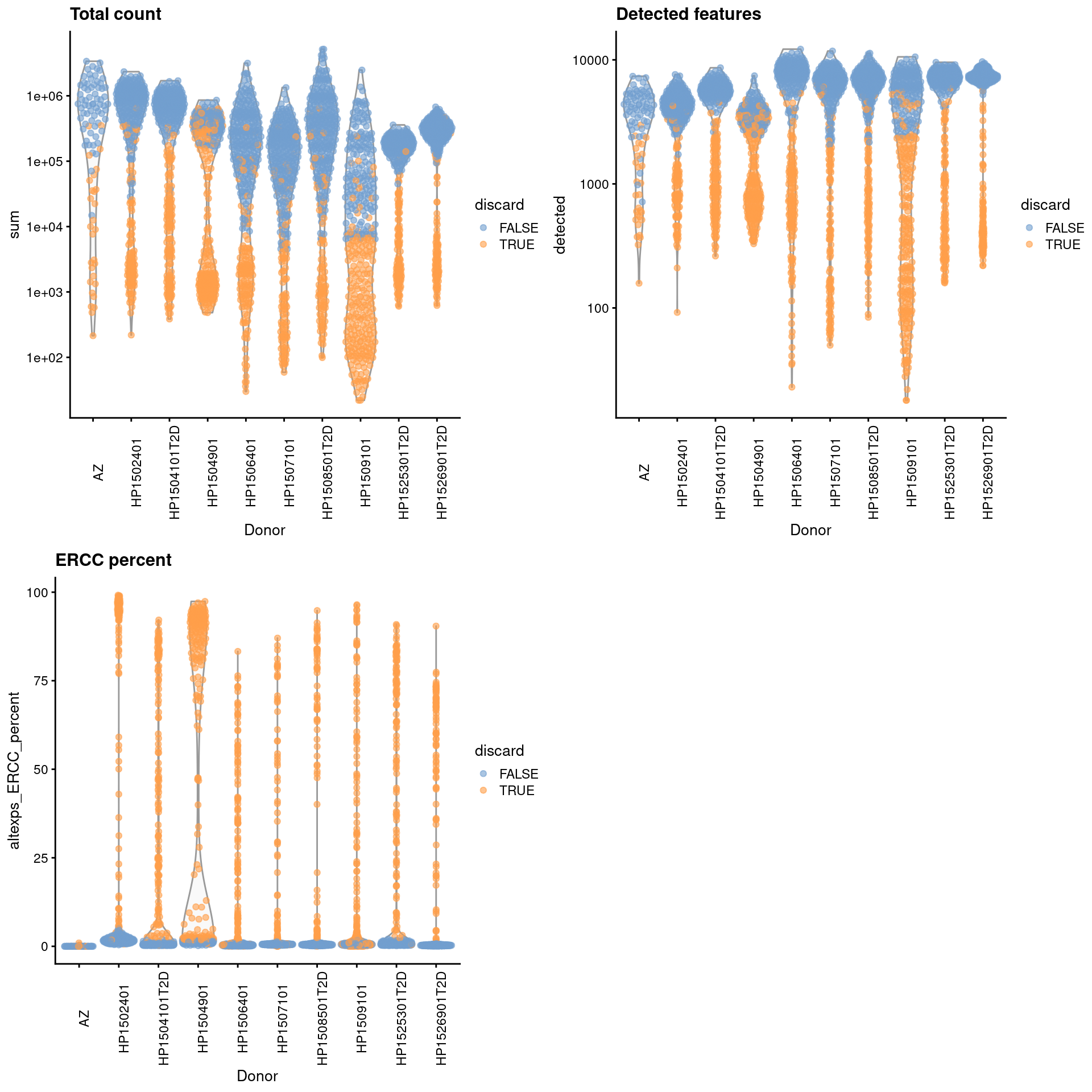
For some batches that seem to have a majority of low-quality cells (Figure \@ref(fig:unref-seger-qc-dist)), we use the other batches to define an appropriate threshold via `subset=`.
```r
low.qual <- sce.seger$Quality == "low quality cell"
library(scater)
stats <- perCellQCMetrics(sce.seger)
qc <- quickPerCellQC(stats, percent_subsets="altexps_ERCC_percent",
batch=sce.seger$Donor,
subset=!sce.seger$Donor %in% c("HP1504901", "HP1509101"))
sce.seger <- sce.seger[,!(qc$discard | low.qual)]
```
```r
colData(unfiltered) <- cbind(colData(unfiltered), stats)
unfiltered$discard <- qc$discard
gridExtra::grid.arrange(
plotColData(unfiltered, x="Donor", y="sum", colour_by="discard") +
scale_y_log10() + ggtitle("Total count") +
theme(axis.text.x = element_text(angle = 90)),
plotColData(unfiltered, x="Donor", y="detected", colour_by="discard") +
scale_y_log10() + ggtitle("Detected features") +
theme(axis.text.x = element_text(angle = 90)),
plotColData(unfiltered, x="Donor", y="altexps_ERCC_percent",
colour_by="discard") + ggtitle("ERCC percent") +
theme(axis.text.x = element_text(angle = 90)),
ncol=2
)
```
(\#fig:unref-seger-qc-dist)Distribution of each QC metric across cells from each donor of the Segerstolpe pancreas dataset. Each point represents a cell and is colored according to whether that cell was discarded.
```r
colSums(as.matrix(qc))
```
```
## low_lib_size low_n_features high_altexps_ERCC_percent
## 788 1056 1031
## discard
## 1246
```
## Normalization
We don't normalize the spike-ins at this point as there are some cells with no spike-in counts.
```r
library(scran)
clusters <- quickCluster(sce.seger)
sce.seger <- computeSumFactors(sce.seger, clusters=clusters)
sce.seger <- logNormCounts(sce.seger)
```
```r
summary(sizeFactors(sce.seger))
```
```
## Min. 1st Qu. Median Mean 3rd Qu. Max.
## 0.014 0.390 0.708 1.000 1.332 11.182
```
```r
plot(librarySizeFactors(sce.seger), sizeFactors(sce.seger), pch=16,
xlab="Library size factors", ylab="Deconvolution factors", log="xy")
```
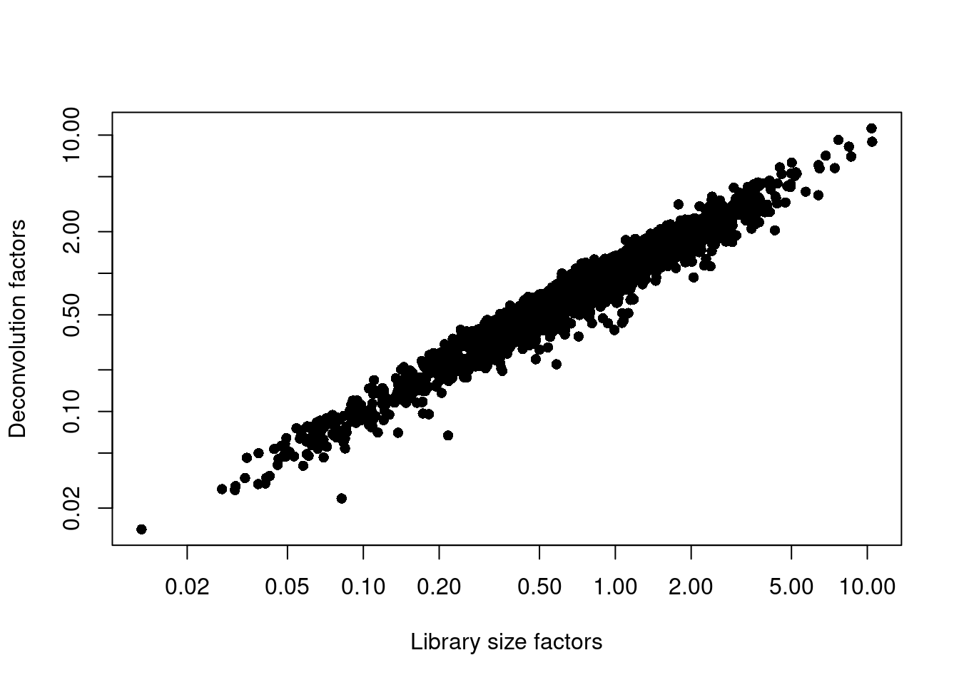
(\#fig:unref-seger-norm)Relationship between the library size factors and the deconvolution size factors in the Segerstolpe pancreas dataset.
## Variance modelling
We do not use cells with no spike-ins for variance modelling.
Donor AZ also has very low spike-in counts and is subsequently ignored.
```r
for.hvg <- sce.seger[,librarySizeFactors(altExp(sce.seger)) > 0 & sce.seger$Donor!="AZ"]
dec.seger <- modelGeneVarWithSpikes(for.hvg, "ERCC", block=for.hvg$Donor)
chosen.hvgs <- getTopHVGs(dec.seger, n=2000)
```
```r
par(mfrow=c(3,3))
blocked.stats <- dec.seger$per.block
for (i in colnames(blocked.stats)) {
current <- blocked.stats[[i]]
plot(current$mean, current$total, main=i, pch=16, cex=0.5,
xlab="Mean of log-expression", ylab="Variance of log-expression")
curfit <- metadata(current)
points(curfit$mean, curfit$var, col="red", pch=16)
curve(curfit$trend(x), col='dodgerblue', add=TRUE, lwd=2)
}
```
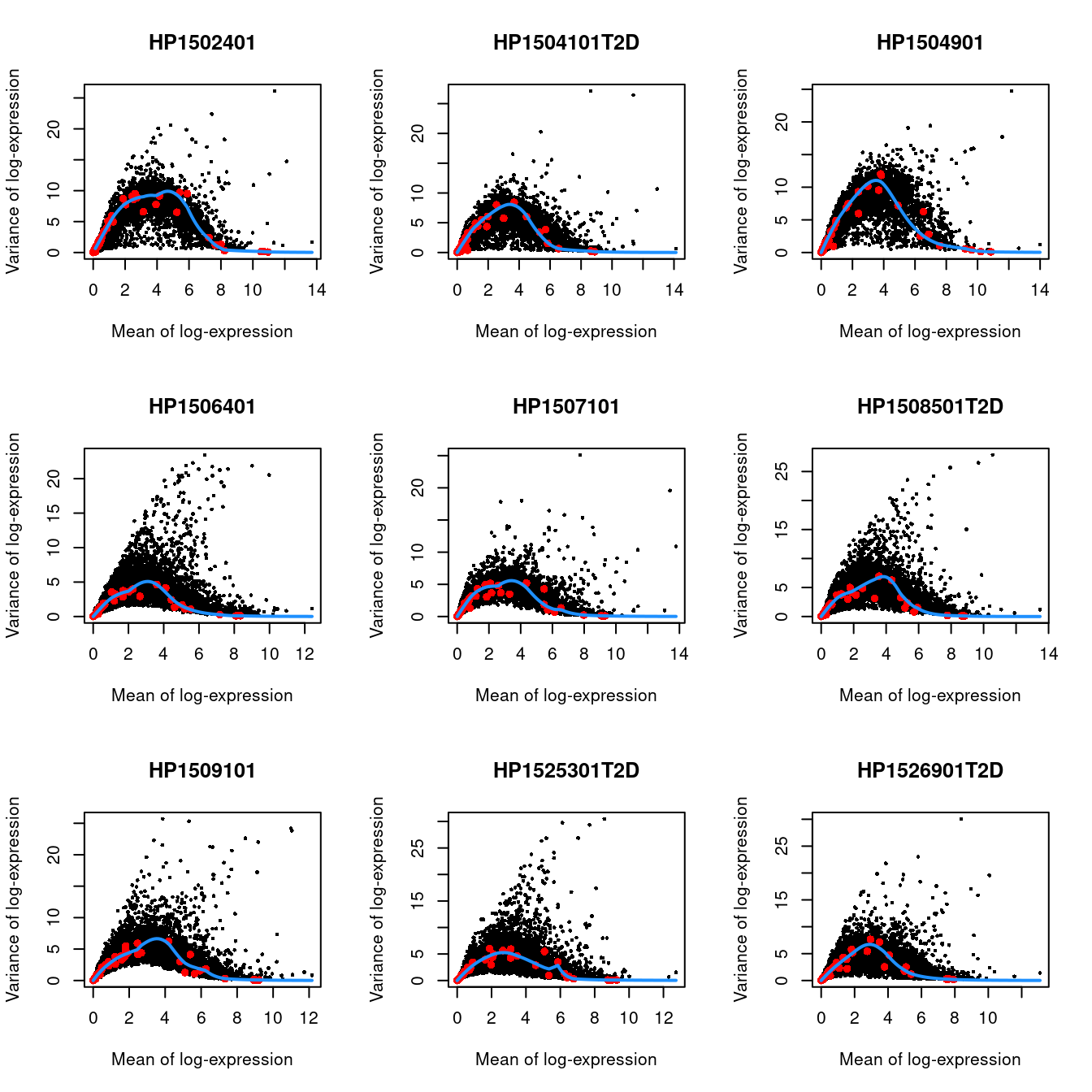
(\#fig:unref-seger-variance)Per-gene variance as a function of the mean for the log-expression values in the Grun pancreas dataset. Each point represents a gene (black) with the mean-variance trend (blue) fitted to the spike-in transcripts (red) separately for each donor.
## Dimensionality reduction
We pick the first 25 PCs for downstream analyses, as it's a nice square number.
```r
library(BiocSingular)
set.seed(101011001)
sce.seger <- runPCA(sce.seger, subset_row=chosen.hvgs, ncomponents=25)
sce.seger <- runTSNE(sce.seger, dimred="PCA")
```
## Clustering
```r
library(bluster)
clust.out <- clusterRows(reducedDim(sce.seger, "PCA"), NNGraphParam(), full=TRUE)
snn.gr <- clust.out$objects$graph
colLabels(sce.seger) <- clust.out$clusters
```
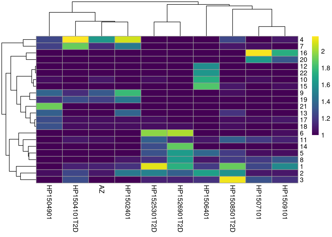
We see a strong donor effect in Figures \@ref(fig:unref-seger-heat-1) and \@ref(fig:unref-grun-tsne).
This might be due to differences in cell type composition between donors,
but the more likely explanation is that of a technical difference in plate processing or uninteresting genotypic differences.
The implication is that we should have called `fastMNN()` at some point.
```r
tab <- table(Cluster=colLabels(sce.seger), Donor=sce.seger$Donor)
library(pheatmap)
pheatmap(log10(tab+10), color=viridis::viridis(100))
```
(\#fig:unref-seger-heat-1)Heatmap of the frequency of cells from each donor in each cluster.
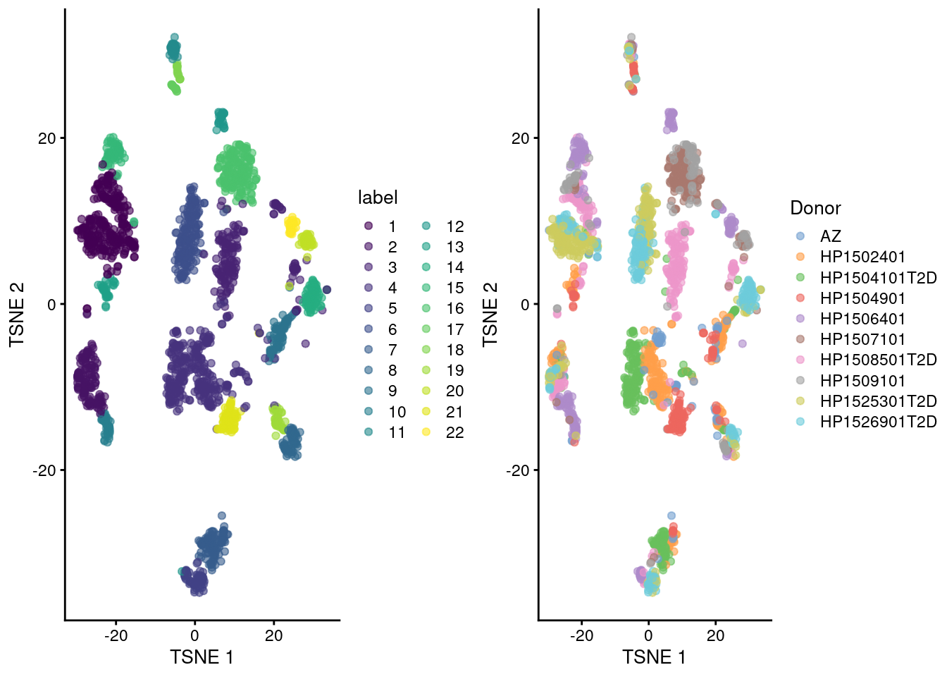
(\#fig:unref-seger-tsne)Obligatory $t$-SNE plots of the Segerstolpe pancreas dataset. Each point represents a cell that is colored by cluster (left) or batch (right).
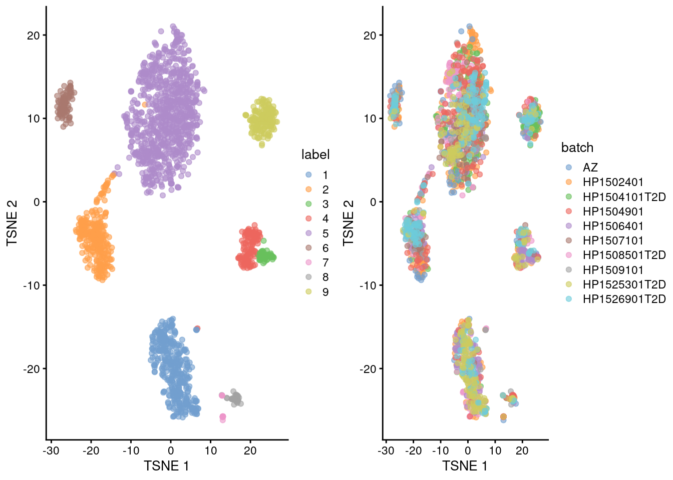
(\#fig:unref-seger-tsne-correct)Yet another $t$-SNE plot of the Segerstolpe dataset, this time after batch correction across donors. Each point represents a cell and is colored by the assigned cluster identity.
## Multi-sample comparisons {#segerstolpe-comparison}
This particular dataset contains both healthy donors and those with type II diabetes.
It is thus of some interest to identify genes that are differentially expressed upon disease in each cell type.
To keep things simple, we use the author-provided annotation rather than determining the cell type for each of our clusters.
```r
summed <- aggregateAcrossCells(sce.seger,
ids=colData(sce.seger)[,c("Donor", "CellType")])
summed
```
```
## class: SingleCellExperiment
## dim: 25454 105
## metadata(0):
## assays(1): counts
## rownames(25454): ENSG00000118473 ENSG00000142920 ... ENSG00000278306
## eGFP
## rowData names(2): symbol refseq
## colnames: NULL
## colData names(9): CellType Disease ... CellType ncells
## reducedDimNames(2): PCA TSNE
## mainExpName: endogenous
## altExpNames(1): ERCC
```
Here, we will use the `voom` pipeline from the *[limma](https://bioconductor.org/packages/3.13/limma)* package instead of the QL approach with *[edgeR](https://bioconductor.org/packages/3.13/edgeR)*.
This allows us to use sample weights to better account for the variation in the precision of each pseudo-bulk profile.
We see that insulin is downregulated in beta cells in the disease state, which is sensible enough.
```r
summed.beta <- summed[,summed$CellType=="Beta"]
library(edgeR)
y.beta <- DGEList(counts(summed.beta), samples=colData(summed.beta),
genes=rowData(summed.beta)[,"symbol",drop=FALSE])
y.beta <- y.beta[filterByExpr(y.beta, group=y.beta$samples$Disease),]
y.beta <- calcNormFactors(y.beta)
design <- model.matrix(~Disease, y.beta$samples)
v.beta <- voomWithQualityWeights(y.beta, design)
fit.beta <- lmFit(v.beta)
fit.beta <- eBayes(fit.beta, robust=TRUE)
res.beta <- topTable(fit.beta, sort.by="p", n=Inf,
coef="Diseasetype II diabetes mellitus")
head(res.beta)
```
```
## symbol logFC AveExpr t P.Value adj.P.Val B
## ENSG00000254647 INS -2.728 16.680 -7.671 3.191e-06 0.03902 4.842
## ENSG00000137731 FXYD2 -2.595 7.265 -6.705 1.344e-05 0.08219 3.353
## ENSG00000169297 NR0B1 -2.092 6.790 -5.789 5.810e-05 0.09916 1.984
## ENSG00000181029 TRAPPC5 -2.127 7.046 -5.678 7.007e-05 0.09916 1.877
## ENSG00000105707 HPN -1.803 6.118 -5.654 7.298e-05 0.09916 1.740
## LOC284889 LOC284889 -2.113 6.652 -5.515 9.259e-05 0.09916 1.571
```
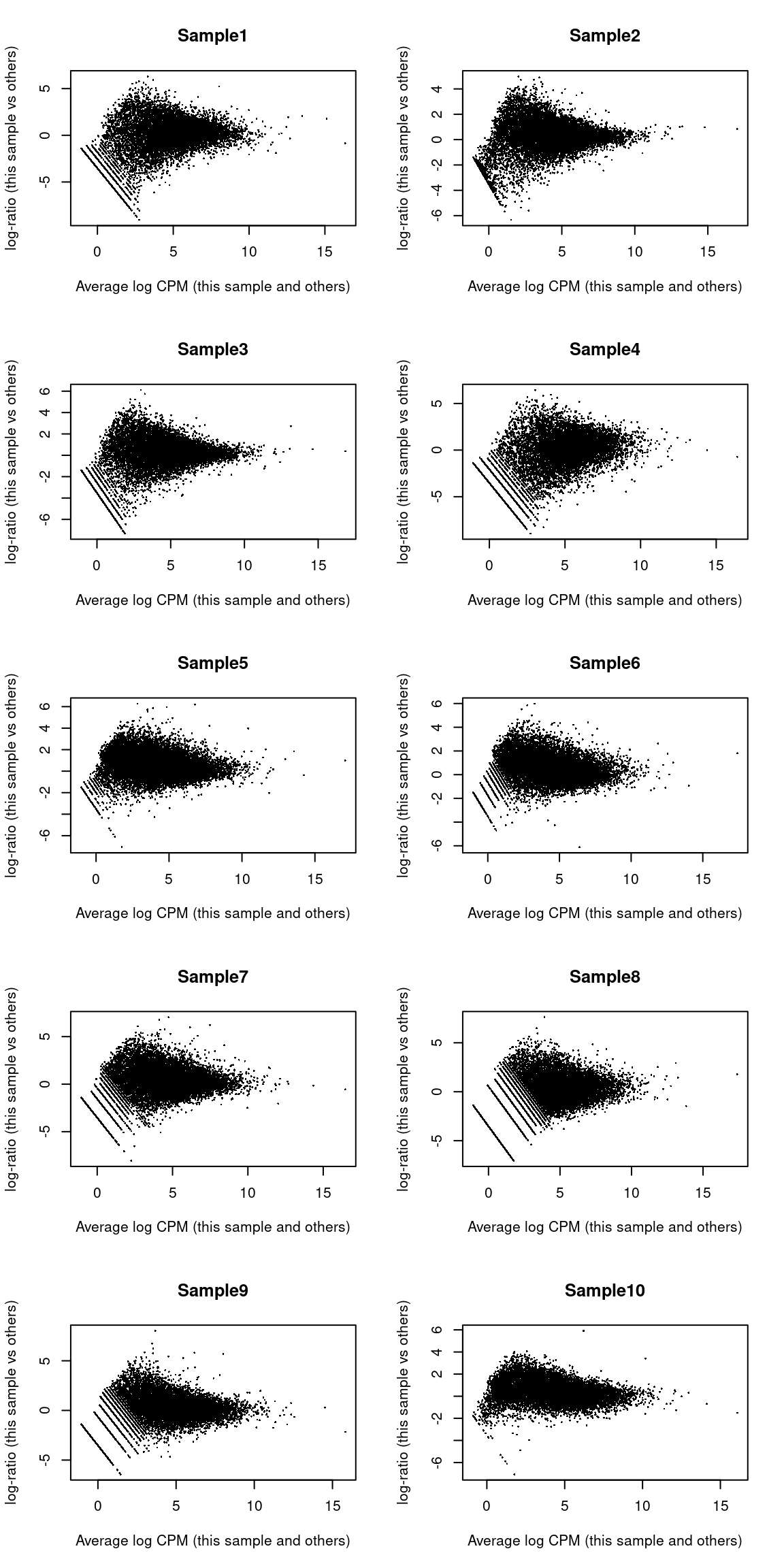
We also create some diagnostic plots to check for potential problems in the analysis.
The MA plots exhibit the expected shape (Figure \@ref(fig:unref-ma-plots))
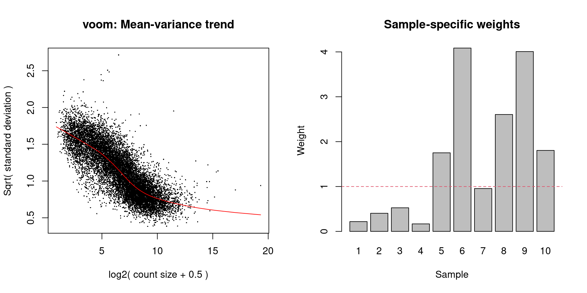
while the differences in the sample weights in Figure \@ref(fig:unref-voom-plots) justify the use of `voom()` in this context.
```r
par(mfrow=c(5, 2))
for (i in colnames(y.beta)) {
plotMD(y.beta, column=i)
}
```
(\#fig:unref-ma-plots)MA plots for the beta cell pseudo-bulk profiles. Each MA plot is generated by comparing the corresponding pseudo-bulk profile against the average of all other profiles
```r
# Easier to just re-run it with plot=TRUE than
# to try to make the plot from 'v.beta'.
voomWithQualityWeights(y.beta, design, plot=TRUE)
```
(\#fig:unref-voom-plots)Diagnostic plots for `voom` after estimating observation and quality weights from the beta cell pseudo-bulk profiles. The left plot shows the mean-variance trend used to estimate the observation weights, while the right plot shows the per-sample quality weights.