# Grun mouse HSC (CEL-seq)
## Introduction
This performs an analysis of the mouse haematopoietic stem cell (HSC) dataset generated with CEL-seq [@grun2016denovo].
Despite its name, this dataset actually contains both sorted HSCs and a population of micro-dissected bone marrow cells.
## Data loading
```r
library(scRNAseq)
sce.grun.hsc <- GrunHSCData(ensembl=TRUE)
```
```r
library(AnnotationHub)
ens.mm.v97 <- AnnotationHub()[["AH73905"]]
anno <- select(ens.mm.v97, keys=rownames(sce.grun.hsc),
keytype="GENEID", columns=c("SYMBOL", "SEQNAME"))
rowData(sce.grun.hsc) <- anno[match(rownames(sce.grun.hsc), anno$GENEID),]
```
After loading and annotation, we inspect the resulting `SingleCellExperiment` object:
```r
sce.grun.hsc
```
```
## class: SingleCellExperiment
## dim: 21817 1915
## metadata(0):
## assays(1): counts
## rownames(21817): ENSMUSG00000109644 ENSMUSG00000007777 ...
## ENSMUSG00000055670 ENSMUSG00000039068
## rowData names(3): GENEID SYMBOL SEQNAME
## colnames(1915): JC4_349_HSC_FE_S13_ JC4_350_HSC_FE_S13_ ...
## JC48P6_1203_HSC_FE_S8_ JC48P6_1204_HSC_FE_S8_
## colData names(2): sample protocol
## reducedDimNames(0):
## mainExpName: NULL
## altExpNames(0):
```
## Quality control
```r
unfiltered <- sce.grun.hsc
```
For some reason, no mitochondrial transcripts are available, and we have no spike-in transcripts, so we only use the number of detected genes and the library size for quality control.
We block on the protocol used for cell extraction, ignoring the micro-dissected cells when computing this threshold.
This is based on our judgement that a majority of micro-dissected plates consist of a majority of low-quality cells, compromising the assumptions of outlier detection.
```r
library(scuttle)
stats <- perCellQCMetrics(sce.grun.hsc)
qc <- quickPerCellQC(stats, batch=sce.grun.hsc$protocol,
subset=grepl("sorted", sce.grun.hsc$protocol))
sce.grun.hsc <- sce.grun.hsc[,!qc$discard]
```
We examine the number of cells discarded for each reason.
```r
colSums(as.matrix(qc))
```
```
## low_lib_size low_n_features discard
## 465 482 488
```
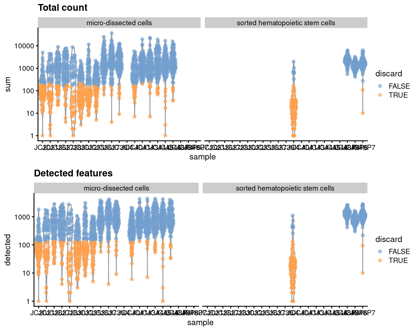
We create some diagnostic plots for each metric (Figure \@ref(fig:unref-hgrun-qc-dist)).
The library sizes are unusually low for many plates of micro-dissected cells; this may be attributable to damage induced by the extraction protocol compared to cell sorting.
```r
colData(unfiltered) <- cbind(colData(unfiltered), stats)
unfiltered$discard <- qc$discard
library(scater)
gridExtra::grid.arrange(
plotColData(unfiltered, y="sum", x="sample", colour_by="discard",
other_fields="protocol") + scale_y_log10() + ggtitle("Total count") +
facet_wrap(~protocol),
plotColData(unfiltered, y="detected", x="sample", colour_by="discard",
other_fields="protocol") + scale_y_log10() +
ggtitle("Detected features") + facet_wrap(~protocol),
ncol=1
)
```
(\#fig:unref-hgrun-qc-dist)Distribution of each QC metric across cells in the Grun HSC dataset. Each point represents a cell and is colored according to whether that cell was discarded.
## Normalization
```r
library(scran)
set.seed(101000110)
clusters <- quickCluster(sce.grun.hsc)
sce.grun.hsc <- computeSumFactors(sce.grun.hsc, clusters=clusters)
sce.grun.hsc <- logNormCounts(sce.grun.hsc)
```
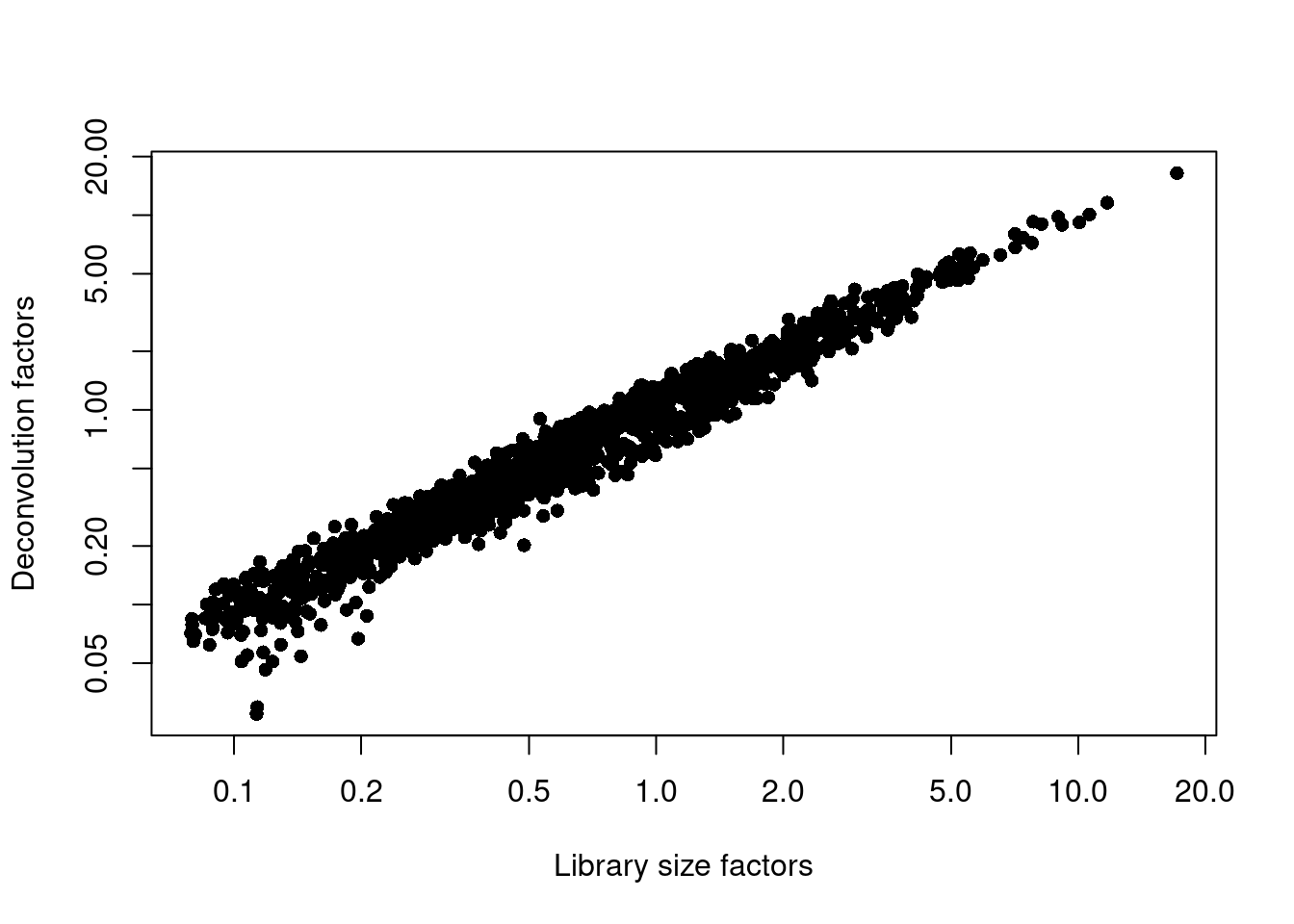
We examine some key metrics for the distribution of size factors, and compare it to the library sizes as a sanity check (Figure \@ref(fig:unref-hgrun-norm)).
```r
summary(sizeFactors(sce.grun.hsc))
```
```
## Min. 1st Qu. Median Mean 3rd Qu. Max.
## 0.027 0.290 0.603 1.000 1.201 16.433
```
```r
plot(librarySizeFactors(sce.grun.hsc), sizeFactors(sce.grun.hsc), pch=16,
xlab="Library size factors", ylab="Deconvolution factors", log="xy")
```
(\#fig:unref-hgrun-norm)Relationship between the library size factors and the deconvolution size factors in the Grun HSC dataset.
## Variance modelling
We create a mean-variance trend based on the expectation that UMI counts have Poisson technical noise.
We do not block on sample here as we want to preserve any difference between the micro-dissected cells and the sorted HSCs.
```r
set.seed(00010101)
dec.grun.hsc <- modelGeneVarByPoisson(sce.grun.hsc)
top.grun.hsc <- getTopHVGs(dec.grun.hsc, prop=0.1)
```
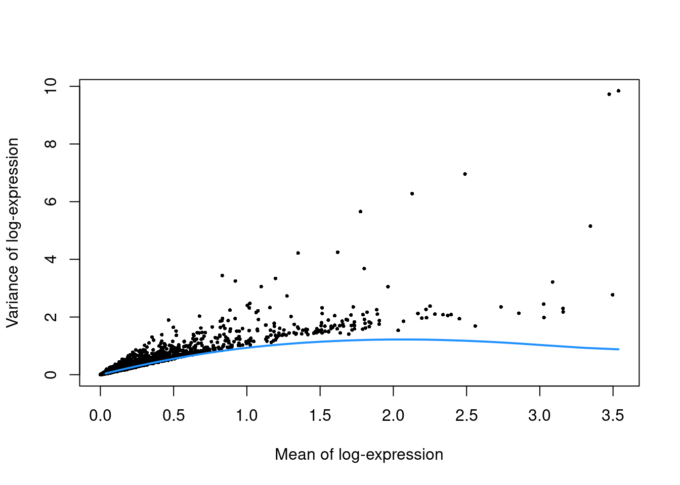
The lack of a typical "bump" shape in Figure \@ref(fig:unref-hgrun-var) is caused by the low counts.
```r
plot(dec.grun.hsc$mean, dec.grun.hsc$total, pch=16, cex=0.5,
xlab="Mean of log-expression", ylab="Variance of log-expression")
curfit <- metadata(dec.grun.hsc)
curve(curfit$trend(x), col='dodgerblue', add=TRUE, lwd=2)
```
(\#fig:unref-hgrun-var)Per-gene variance as a function of the mean for the log-expression values in the Grun HSC dataset. Each point represents a gene (black) with the mean-variance trend (blue) fitted to the simulated Poisson-distributed noise.
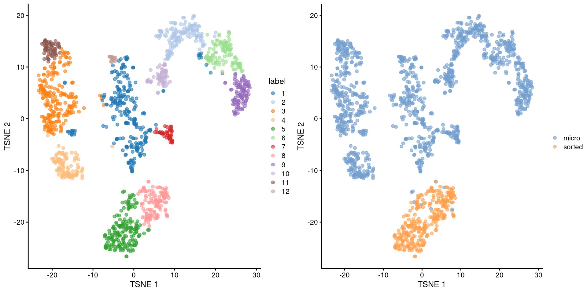
(\#fig:unref-hgrun-tsne)Obligatory $t$-SNE plot of the Grun HSC dataset, where each point represents a cell and is colored according to the assigned cluster (left) or extraction protocol (right).
## Marker gene detection
```r
markers <- findMarkers(sce.grun.hsc, test.type="wilcox", direction="up",
row.data=rowData(sce.grun.hsc)[,"SYMBOL",drop=FALSE])
```
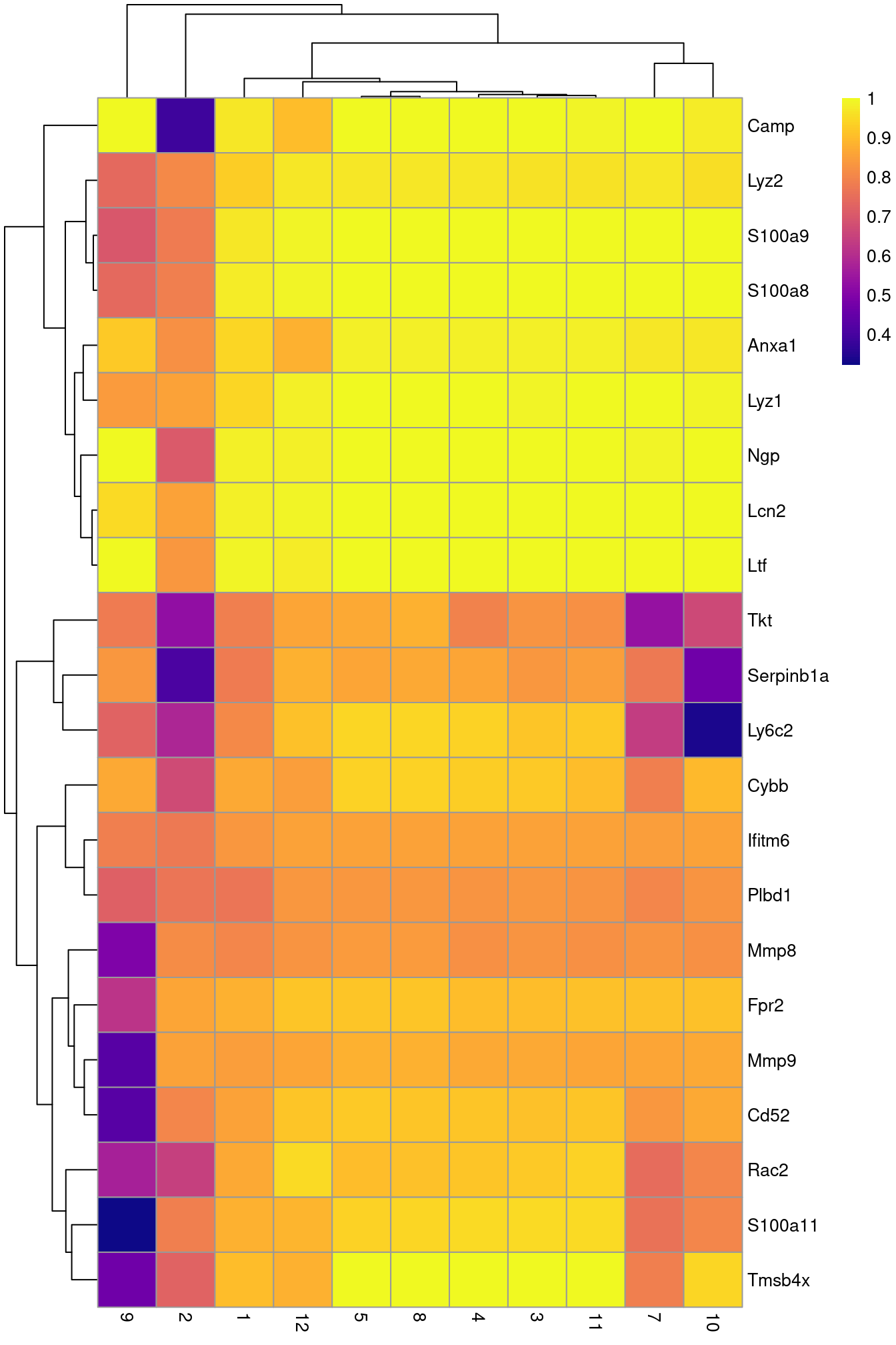
To illustrate the manual annotation process, we examine the marker genes for one of the clusters.
Upregulation of _Camp_, _Lcn2_, _Ltf_ and lysozyme genes indicates that this cluster contains cells of neuronal origin.
```r
chosen <- markers[['6']]
best <- chosen[chosen$Top <= 10,]
aucs <- getMarkerEffects(best, prefix="AUC")
rownames(aucs) <- best$SYMBOL
library(pheatmap)
pheatmap(aucs, color=viridis::plasma(100))
```
(\#fig:unref-heat-hgrun-markers)Heatmap of the AUCs for the top marker genes in cluster 6 compared to all other clusters in the Grun HSC dataset.