# Messmer human ESC (Smart-seq2) {#messmer-hesc}
## Introduction
This performs an analysis of the human embryonic stem cell (hESC) dataset generated with Smart-seq2 [@messmer2019transcriptional], which contains several plates of naive and primed hESCs.
The chapter's code is based on the steps in the paper's [GitHub repository](https://github.com/MarioniLab/NaiveHESC2016/blob/master/analysis/preprocess.Rmd), with some additional steps for cell cycle effect removal contributed by Philippe Boileau.
## Data loading
Converting the batch to a factor, to make life easier later on.
```r
library(scRNAseq)
sce.mess <- MessmerESCData()
sce.mess$`experiment batch` <- factor(sce.mess$`experiment batch`)
```
```r
library(AnnotationHub)
ens.hs.v97 <- AnnotationHub()[["AH73881"]]
anno <- select(ens.hs.v97, keys=rownames(sce.mess),
keytype="GENEID", columns=c("SYMBOL"))
rowData(sce.mess) <- anno[match(rownames(sce.mess), anno$GENEID),]
```
## Quality control
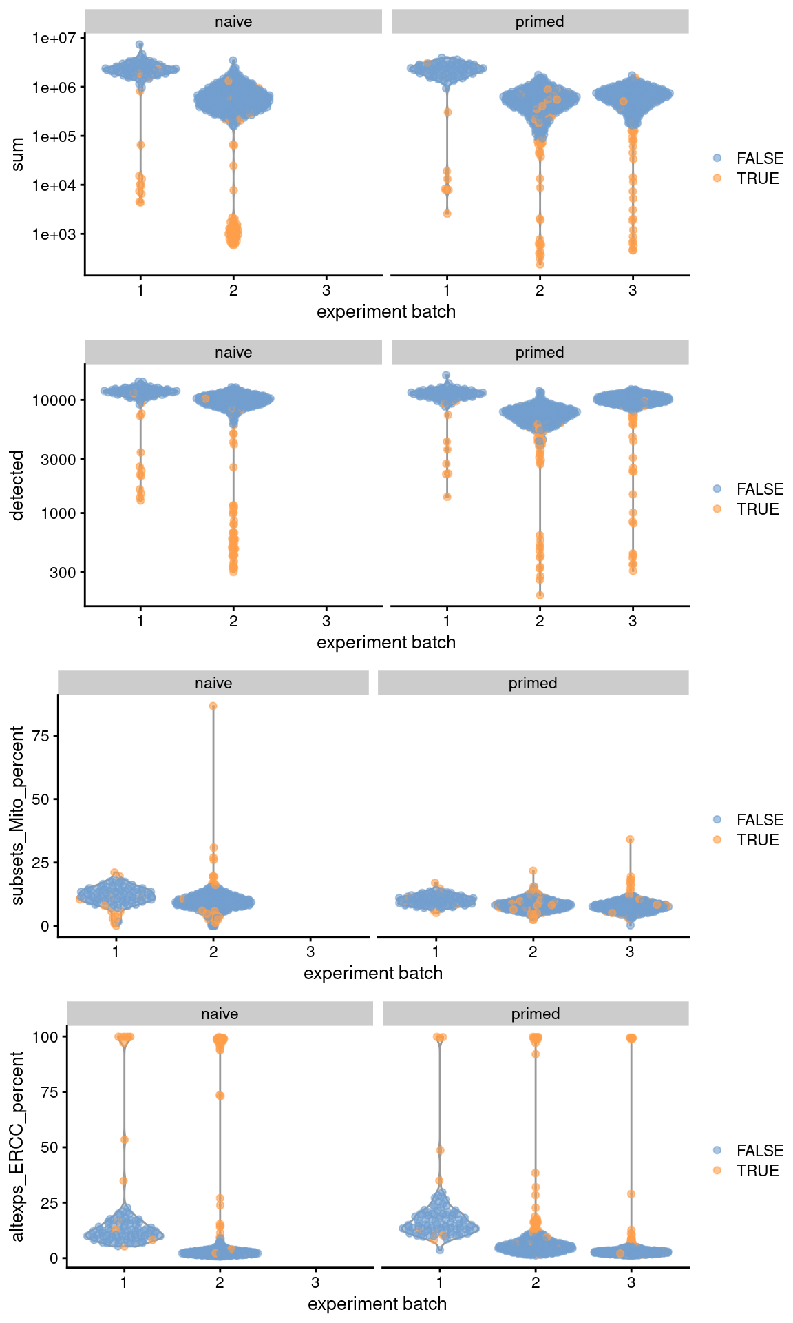
Let's have a look at the QC statistics.
```r
colSums(as.matrix(filtered))
```
```
## low_lib_size low_n_features high_subsets_Mito_percent
## 107 99 22
## high_altexps_ERCC_percent discard
## 117 156
```
```r
gridExtra::grid.arrange(
plotColData(original, x="experiment batch", y="sum",
colour_by=I(filtered$discard), other_field="phenotype") +
facet_wrap(~phenotype) + scale_y_log10(),
plotColData(original, x="experiment batch", y="detected",
colour_by=I(filtered$discard), other_field="phenotype") +
facet_wrap(~phenotype) + scale_y_log10(),
plotColData(original, x="experiment batch", y="subsets_Mito_percent",
colour_by=I(filtered$discard), other_field="phenotype") +
facet_wrap(~phenotype),
plotColData(original, x="experiment batch", y="altexps_ERCC_percent",
colour_by=I(filtered$discard), other_field="phenotype") +
facet_wrap(~phenotype),
ncol=1
)
```
(\#fig:unref-messmer-hesc-qc)Distribution of QC metrics across batches (x-axis) and phenotypes (facets) for cells in the Messmer hESC dataset. Each point is a cell and is colored by whether it was discarded.
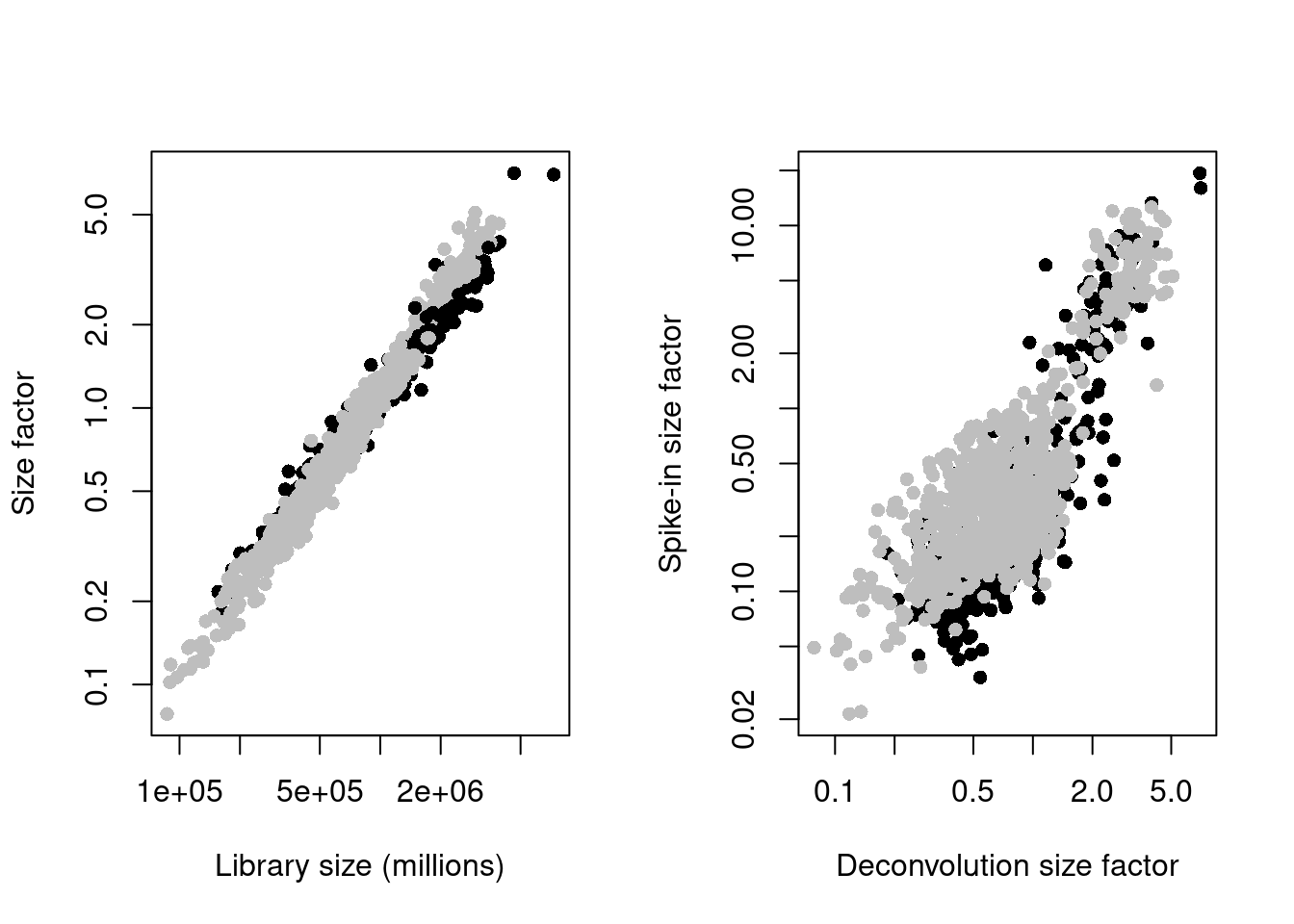
(\#fig:unref-messmer-hesc-norm)Deconvolution size factors plotted against the library size (left) and spike-in size factors plotted against the deconvolution size factors (right). Each point is a cell and is colored by its phenotype.
## Cell cycle phase assignment
Here, we use multiple cores to speed up the processing.
```r
set.seed(10001)
hs_pairs <- readRDS(system.file("exdata", "human_cycle_markers.rds", package="scran"))
assigned <- cyclone(sce.mess, pairs=hs_pairs,
gene.names=rownames(sce.mess),
BPPARAM=BiocParallel::MulticoreParam(10))
sce.mess$phase <- assigned$phases
```
```r
table(sce.mess$phase)
```
```
##
## G1 G2M S
## 460 406 322
```
```r
smoothScatter(assigned$scores$G1, assigned$scores$G2M, xlab="G1 score",
ylab="G2/M score", pch=16)
```
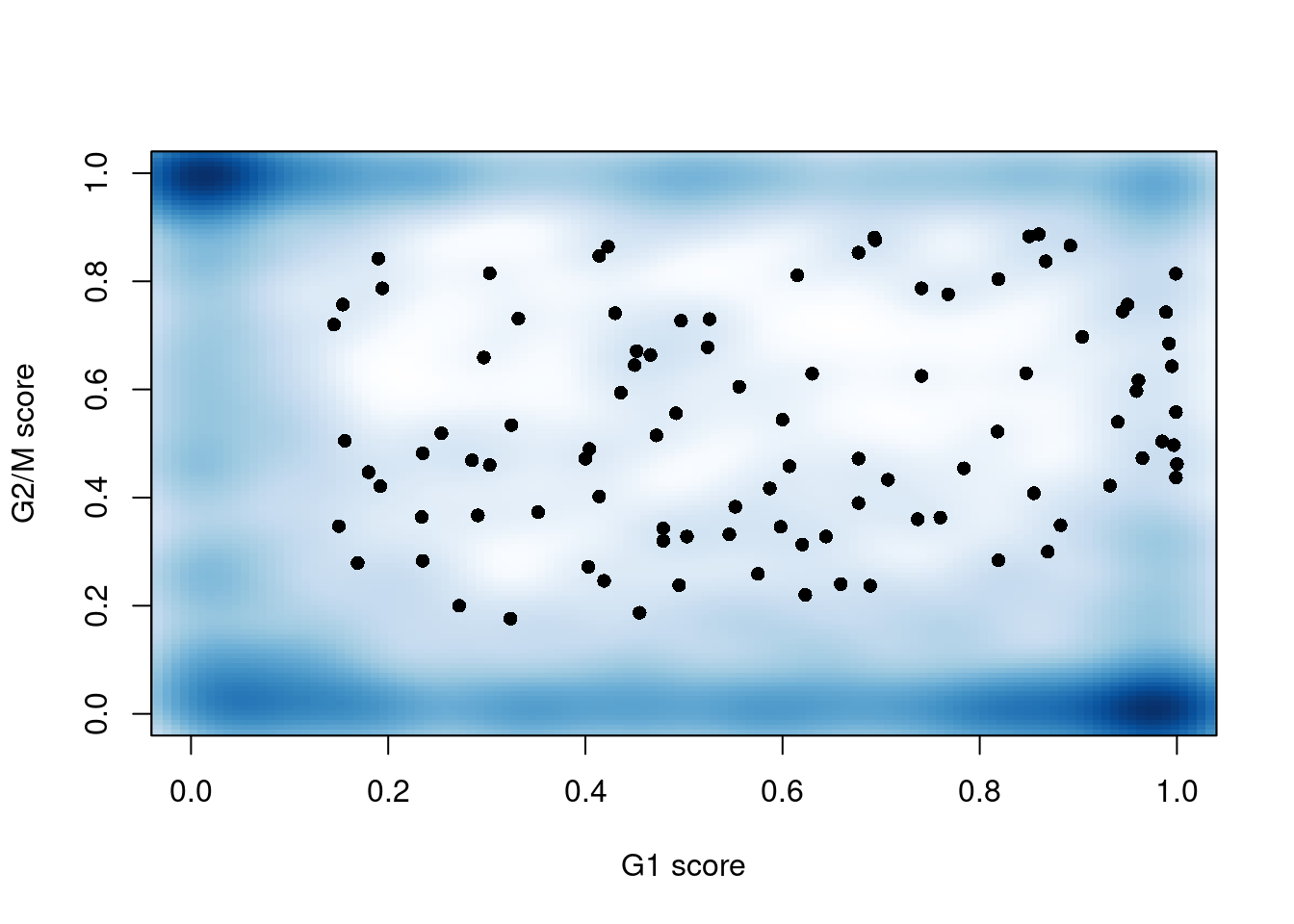
(\#fig:unref-messmer-hesc-cyclone)G1 `cyclone()` phase scores against the G2/M phase scores for each cell in the Messmer hESC dataset.
## Feature selection
```r
dec <- modelGeneVarWithSpikes(sce.mess, "ERCC", block = sce.mess$`experiment batch`)
top.hvgs <- getTopHVGs(dec, prop = 0.1)
```
```r
par(mfrow=c(1,3))
for (i in seq_along(dec$per.block)) {
current <- dec$per.block[[i]]
plot(current$mean, current$total, xlab="Mean log-expression",
ylab="Variance", pch=16, cex=0.5, main=paste("Batch", i))
fit <- metadata(current)
points(fit$mean, fit$var, col="red", pch=16)
curve(fit$trend(x), col='dodgerblue', add=TRUE, lwd=2)
}
```
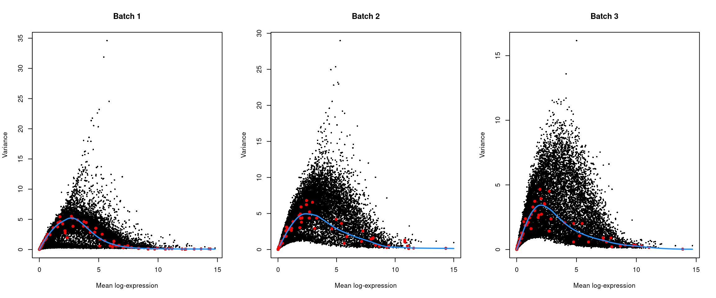
(\#fig:unref-messmer-hesc-var)Per-gene variance of the log-normalized expression values in the Messmer hESC dataset, plotted against the mean for each batch. Each point represents a gene with spike-ins shown in red and the fitted trend shown in blue.
## Batch correction
We eliminate the obvious batch effect between batches with linear regression, which is possible due to the replicated nature of the experimental design.
We set `keep=1:2` to retain the effect of the first two coefficients in `design` corresponding to our phenotype of interest.
```r
library(batchelor)
sce.mess <- correctExperiments(sce.mess,
PARAM = RegressParam(
design = model.matrix(~sce.mess$phenotype + sce.mess$`experiment batch`),
keep = 1:2
)
)
```
## Dimensionality Reduction
We could have set `d=` and `subset.row=` in `correctExperiments()` to automatically perform a PCA on the the residual matrix with the subset of HVGs,
but we'll just explicitly call `runPCA()` here to keep things simple.
```r
set.seed(1101001)
sce.mess <- runPCA(sce.mess, subset_row = top.hvgs, exprs_values = "corrected")
sce.mess <- runTSNE(sce.mess, dimred = "PCA", perplexity = 40)
```
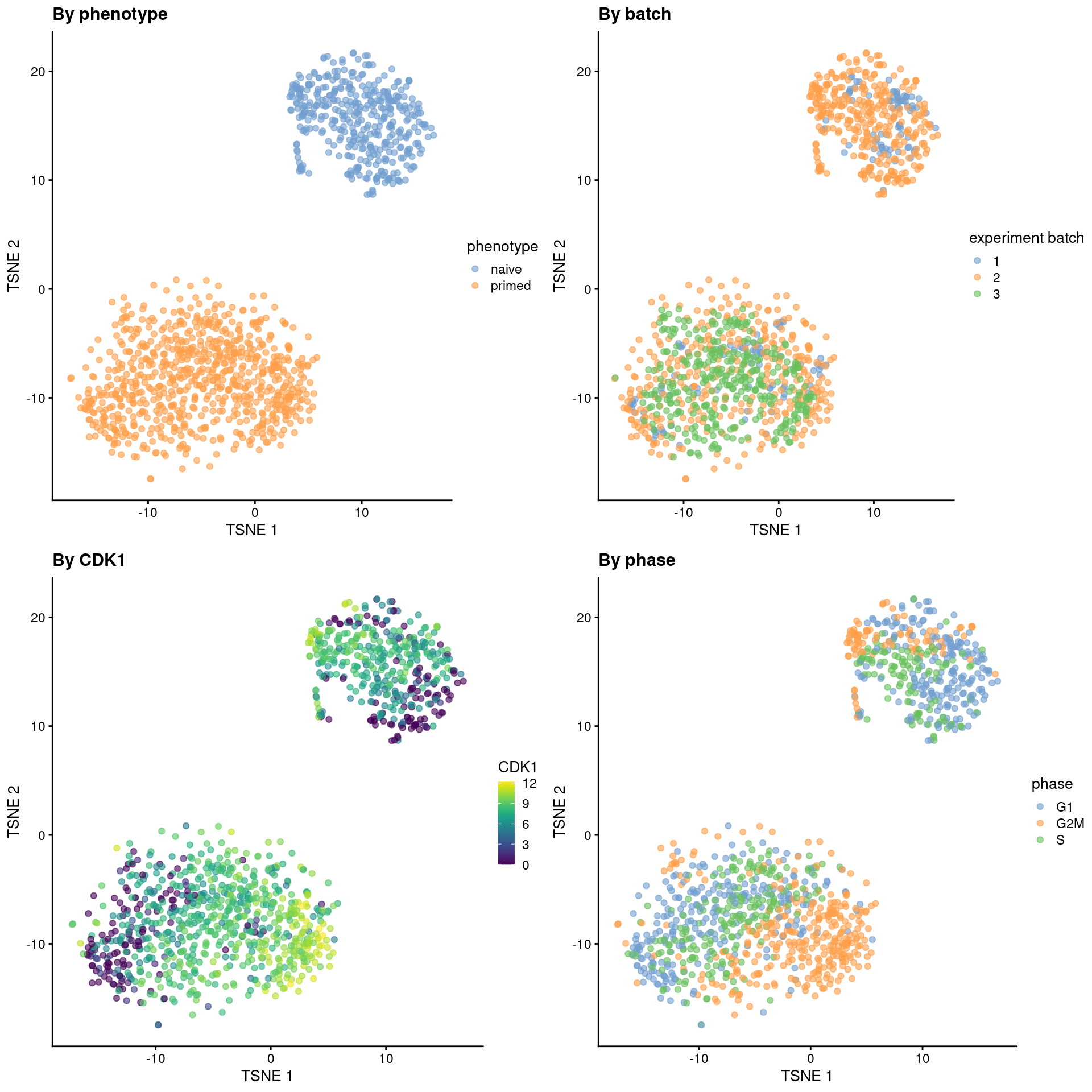
From a naive PCA, the cell cycle appears to be a major source of biological variation within each phenotype.
```r
gridExtra::grid.arrange(
plotTSNE(sce.mess, colour_by = "phenotype") + ggtitle("By phenotype"),
plotTSNE(sce.mess, colour_by = "experiment batch") + ggtitle("By batch "),
plotTSNE(sce.mess, colour_by = "CDK1", swap_rownames="SYMBOL") + ggtitle("By CDK1"),
plotTSNE(sce.mess, colour_by = "phase") + ggtitle("By phase"),
ncol = 2
)
```
(\#fig:unref-messmer-hesc-tsne)Obligatory $t$-SNE plots of the Messmer hESC dataset, where each point is a cell and is colored by various attributes.
We perform contrastive PCA (cPCA) and sparse cPCA (scPCA) on the corrected log-expression data to obtain the same number of PCs.
Given that the naive hESCs are actually reprogrammed primed hESCs, we will use the single batch of primed-only hESCs as the "background" dataset to remove the cell cycle effect.
```r
library(scPCA)
is.bg <- sce.mess$`experiment batch`=="3"
target <- sce.mess[,!is.bg]
background <- sce.mess[,is.bg]
mat.target <- t(assay(target, "corrected")[top.hvgs,])
mat.background <- t(assay(background, "corrected")[top.hvgs,])
set.seed(1010101001)
con_out <- scPCA(
target = mat.target,
background = mat.background,
penalties = 0, # no penalties = non-sparse cPCA.
n_eigen = 50,
contrasts = 100
)
reducedDim(target, "cPCA") <- con_out$x
```
```r
set.seed(101010101)
sparse_con_out <- scPCA(
target = mat.target,
background = mat.background,
penalties = 1e-4,
n_eigen = 50,
contrasts = 100,
alg = "rand_var_proj" # for speed.
)
reducedDim(target, "scPCA") <- sparse_con_out$x
```
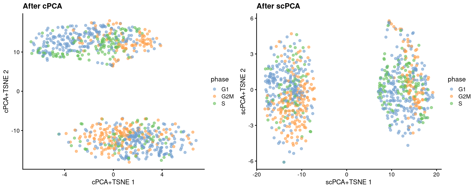
We see greater intermingling between phases within both the naive and primed cells after cPCA and scPCA.
```r
set.seed(1101001)
target <- runTSNE(target, dimred = "cPCA", perplexity = 40, name="cPCA+TSNE")
target <- runTSNE(target, dimred = "scPCA", perplexity = 40, name="scPCA+TSNE")
```
```r
gridExtra::grid.arrange(
plotReducedDim(target, "cPCA+TSNE", colour_by = "phase") + ggtitle("After cPCA"),
plotReducedDim(target, "scPCA+TSNE", colour_by = "phase") + ggtitle("After scPCA"),
ncol=2
)
```
(\#fig:unref-messmer-hesc-cpca-tsne)More $t$-SNE plots of the Messmer hESC dataset after cPCA and scPCA, where each point is a cell and is colored by its assigned cell cycle phase.
We can quantify the change in the separation between phases within each phenotype using the silhouette coefficient.
```r
library(bluster)
naive <- target[,target$phenotype=="naive"]
primed <- target[,target$phenotype=="primed"]
N <- approxSilhouette(reducedDim(naive, "PCA"), naive$phase)
P <- approxSilhouette(reducedDim(primed, "PCA"), primed$phase)
c(naive=mean(N$width), primed=mean(P$width))
```
```
## naive primed
## 0.02032 0.03025
```
```r
cN <- approxSilhouette(reducedDim(naive, "cPCA"), naive$phase)
cP <- approxSilhouette(reducedDim(primed, "cPCA"), primed$phase)
c(naive=mean(cN$width), primed=mean(cP$width))
```
```
## naive primed
## 0.007696 0.011941
```
```r
scN <- approxSilhouette(reducedDim(naive, "scPCA"), naive$phase)
scP <- approxSilhouette(reducedDim(primed, "scPCA"), primed$phase)
c(naive=mean(scN$width), primed=mean(scP$width))
```
```
## naive primed
## 0.006614 0.014601
```
## Session Info {-}