---
output: html_document
bibliography: ref.bib
---
# Cell type annotation
## Motivation
The most challenging task in scRNA-seq data analysis is arguably the interpretation of the results.
Obtaining clusters of cells is fairly straightforward, but it is more difficult to determine what biological state is represented by each of those clusters.
Doing so requires us to bridge the gap between the current dataset and prior biological knowledge, and the latter is not always available in a consistent and quantitative manner.
Indeed, even the concept of a "cell type" is [not clearly defined](https://doi.org/10.1016/j.cels.2017.03.006), with most practitioners possessing a "I'll know it when I see it" intuition that is not amenable to computational analysis.
As such, interpretation of scRNA-seq data is often manual and a common bottleneck in the analysis workflow.
To expedite this step, we can use various computational approaches that exploit prior information to assign meaning to an uncharacterized scRNA-seq dataset.
The most obvious sources of prior information are the curated gene sets associated with particular biological processes, e.g., from the Gene Ontology (GO) or the Kyoto Encyclopedia of Genes and Genomes (KEGG) collections.
Alternatively, we can directly compare our expression profiles to published reference datasets where each sample or cell has already been annotated with its putative biological state by domain experts.
Here, we will demonstrate both approaches with several different scRNA-seq datasets.
## Assigning cell labels from reference data
### Overview
A conceptually straightforward annotation approach is to compare the single-cell expression profiles with previously annotated reference datasets.
Labels can then be assigned to each cell in our uncharacterized test dataset based on the most similar reference sample(s), for some definition of "similar".
This is a standard classification challenge that can be tackled by standard machine learning techniques such as random forests and support vector machines.
Any published and labelled RNA-seq dataset (bulk or single-cell) can be used as a reference, though its reliability depends greatly on the expertise of the original authors who assigned the labels in the first place.
In this section, we will demonstrate the use of the *[SingleR](https://bioconductor.org/packages/3.12/SingleR)* method [@aran2019reference] for cell type annotation.
This method assigns labels to cells based on the reference samples with the highest Spearman rank correlations, using only the marker genes between pairs of labels to focus on the relevant differences between cell types.
It also performs a fine-tuning step for each cell where the correlations are recomputed with just the marker genes for the top-scoring labels.
This aims to resolve any ambiguity between those labels by removing noise from irrelevant markers for other labels.
Further details can be found in the [_SingleR_ book](https://ltla.github.io/SingleRBook) from which most of the examples here are derived.
### Using existing references
For demonstration purposes, we will use one of the 10X PBMC datasets as our test.
While we have already applied quality control, normalization and clustering for this dataset, this is not strictly necessary.
It is entirely possible to run `SingleR()` on the raw counts without any _a priori_ quality control
and filter on the annotation results at one's leisure - see the book for an explanation.
```r
sce.pbmc
```
```
## class: SingleCellExperiment
## dim: 33694 3985
## metadata(1): Samples
## assays(2): counts logcounts
## rownames(33694): RP11-34P13.3 FAM138A ... AC213203.1 FAM231B
## rowData names(2): ID Symbol
## colnames(3985): AAACCTGAGAAGGCCT-1 AAACCTGAGACAGACC-1 ...
## TTTGTCAGTTAAGACA-1 TTTGTCATCCCAAGAT-1
## colData names(4): Sample Barcode sizeFactor label
## reducedDimNames(3): PCA TSNE UMAP
## altExpNames(0):
```
The *[celldex](https://bioconductor.org/packages/3.12/celldex)* contains a number of curated reference datasets, mostly assembled from bulk RNA-seq or microarray data of sorted cell types.
These references are often good enough for most applications provided that they contain the cell types that are expected in the test population.
Here, we will use a reference constructed from Blueprint and ENCODE data [@martens2013blueprint;@encode2012integrated];
this is obtained by calling the `BlueprintEncode()` function to construct a `SummarizedExperiment` containing log-expression values with curated labels for each sample.
```r
library(celldex)
ref <- BlueprintEncodeData()
ref
```
```
## class: SummarizedExperiment
## dim: 19859 259
## metadata(0):
## assays(1): logcounts
## rownames(19859): TSPAN6 TNMD ... LINC00550 GIMAP1-GIMAP5
## rowData names(0):
## colnames(259): mature.neutrophil
## CD14.positive..CD16.negative.classical.monocyte ...
## epithelial.cell.of.umbilical.artery.1
## dermis.lymphatic.vessel.endothelial.cell.1
## colData names(3): label.main label.fine label.ont
```
We call the `SingleR()` function to annotate each of our PBMCs with the main cell type labels from the Blueprint/ENCODE reference.
This returns a `DataFrame` where each row corresponds to a cell in the test dataset and contains its label assignments.
Alternatively, we could use the labels in `ref$label.fine`, which provide more resolution at the cost of speed and increased ambiguity in the assignments.
```r
library(SingleR)
pred <- SingleR(test=sce.pbmc, ref=ref, labels=ref$label.main)
table(pred$labels)
```
```
##
## B-cells CD4+ T-cells CD8+ T-cells DC Eosinophils Erythrocytes
## 549 773 1274 1 1 5
## HSC Monocytes NK cells
## 14 1117 251
```
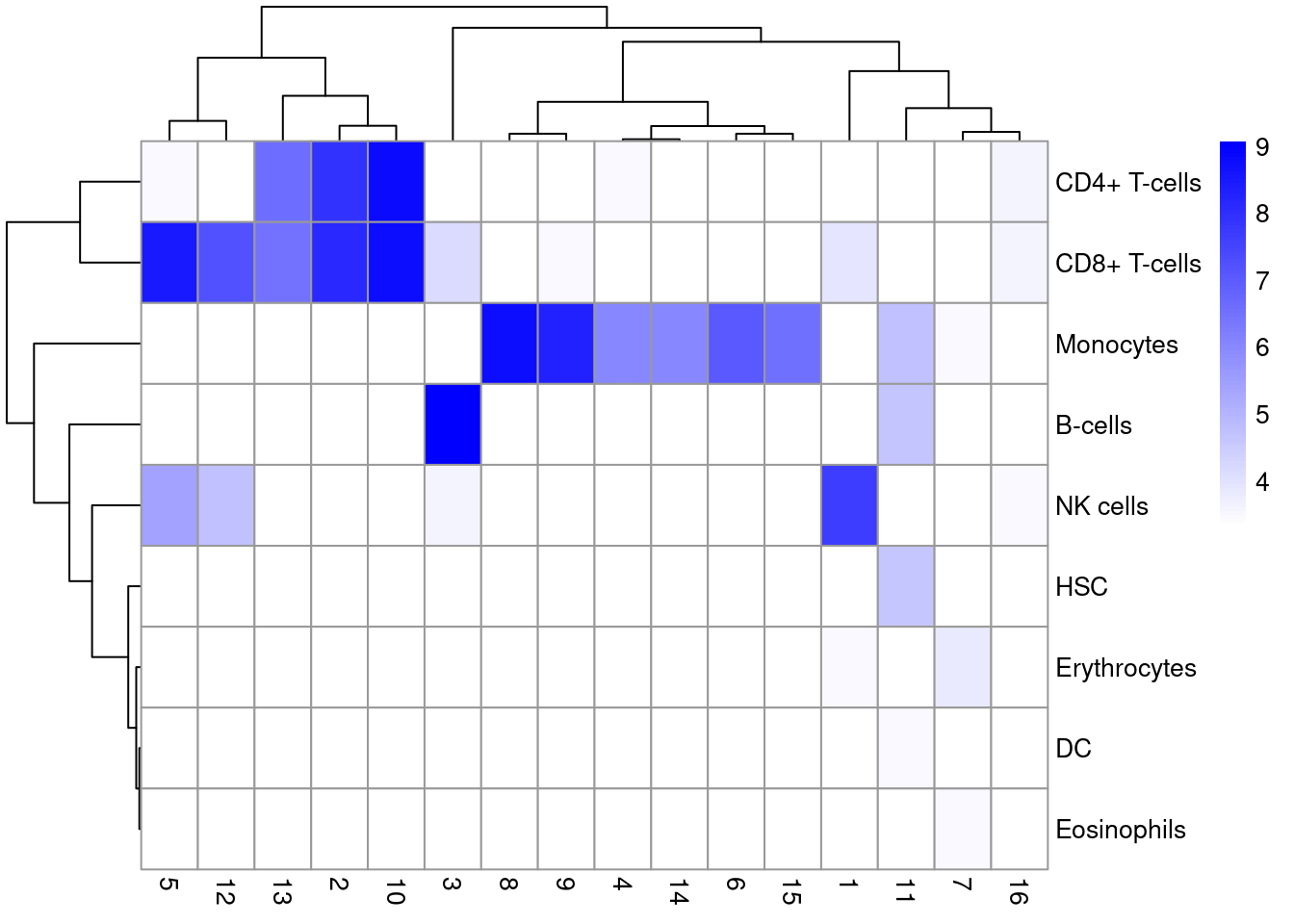
We inspect the results using a heatmap of the per-cell and label scores (Figure \@ref(fig:singler-heat-pbmc)).
Ideally, each cell should exhibit a high score in one label relative to all of the others, indicating that the assignment to that label was unambiguous.
This is largely the case for monocytes and B cells, whereas we see more ambiguity between CD4^+^ and CD8^+^ T cells (and to a lesser extent, NK cells).
```r
plotScoreHeatmap(pred)
```
(\#fig:singler-heat-pbmc)Heatmap of the assignment score for each cell (column) and label (row). Scores are shown before any fine-tuning and are normalized to [0, 1] within each cell.
We compare the assignments with the clustering results to determine the identity of each cluster.
Here, several clusters are nested within the monocyte and B cell labels (Figure \@ref(fig:singler-cluster)), indicating that the clustering represents finer subdivisions within the cell types.
Interestingly, our clustering does not effectively distinguish between CD4^+^ and CD8^+^ T cell labels.
This is probably due to the presence of other factors of heterogeneity within the T cell subpopulation (e.g., activation) that have a stronger influence on unsupervised methods than the _a priori_ expected CD4^+^/CD8^+^ distinction.
```r
tab <- table(Assigned=pred$pruned.labels, Cluster=colLabels(sce.pbmc))
# Adding a pseudo-count of 10 to avoid strong color jumps with just 1 cell.
library(pheatmap)
pheatmap(log2(tab+10), color=colorRampPalette(c("white", "blue"))(101))
```
(\#fig:singler-cluster)Heatmap of the distribution of cells across labels and clusters in the 10X PBMC dataset. Color scale is reported in the log~10~-number of cells for each cluster-label combination.
This episode highlights some of the differences between reference-based annotation and unsupervised clustering.
The former explicitly focuses on aspects of the data that are known to be interesting, simplifying the process of biological interpretation.
However, the cost is that the downstream analysis is restricted by the diversity and resolution of the available labels, a problem that is largely avoided by _de novo_ identification of clusters.
We suggest applying both strategies to examine the agreement (or lack thereof) between reference label and cluster assignments.
Any inconsistencies are not necessarily problematic due to the conceptual differences between the two approaches;
indeed, one could use those discrepancies as the basis for further investigation to discover novel factors of variation in the data.
### Using custom references
We can also apply *[SingleR](https://bioconductor.org/packages/3.12/SingleR)* to single-cell reference datasets that are curated and supplied by the user.
This is most obviously useful when we have an existing dataset that was previously (manually) annotated
and we want to use that knowledge to annotate a new dataset in an automated manner.
To illustrate, we will use the @muraro2016singlecell human pancreas dataset as our reference.
```r
sce.muraro
```
```
## class: SingleCellExperiment
## dim: 16940 2299
## metadata(0):
## assays(2): counts logcounts
## rownames(16940): ENSG00000268895 ENSG00000121410 ... ENSG00000159840
## ENSG00000074755
## rowData names(2): symbol chr
## colnames(2299): D28-1_1 D28-1_2 ... D30-8_93 D30-8_94
## colData names(4): label donor plate sizeFactor
## reducedDimNames(0):
## altExpNames(1): ERCC
```
```r
# Pruning out unknown or unclear labels.
sce.muraro <- sce.muraro[,!is.na(sce.muraro$label) &
sce.muraro$label!="unclear"]
table(sce.muraro$label)
```
```
##
## acinar alpha beta delta duct endothelial
## 217 795 442 189 239 18
## epsilon mesenchymal pp
## 3 80 96
```
Our aim is to assign labels to our test dataset from @segerstolpe2016singlecell.
We use the same call to `SingleR()` but with `de.method="wilcox"` to identify markers via pairwise Wilcoxon ranked sum tests between labels in the reference Muraro dataset.
This re-uses the same machinery from Chapter \@ref(marker-detection); further options to fine-tune the test procedure can be passed via the `de.args` argument.
```r
# Converting to FPKM for a more like-for-like comparison to UMI counts.
# However, results are often still good even when this step is skipped.
library(AnnotationHub)
hs.db <- AnnotationHub()[["AH73881"]]
hs.exons <- exonsBy(hs.db, by="gene")
hs.exons <- reduce(hs.exons)
hs.len <- sum(width(hs.exons))
library(scuttle)
available <- intersect(rownames(sce.seger), names(hs.len))
fpkm.seger <- calculateFPKM(sce.seger[available,], hs.len[available])
pred.seger <- SingleR(test=fpkm.seger, ref=sce.muraro,
labels=sce.muraro$label, de.method="wilcox")
table(pred.seger$labels)
```
```
##
## acinar alpha beta delta duct endothelial
## 192 892 273 106 381 18
## epsilon mesenchymal pp
## 5 52 171
```
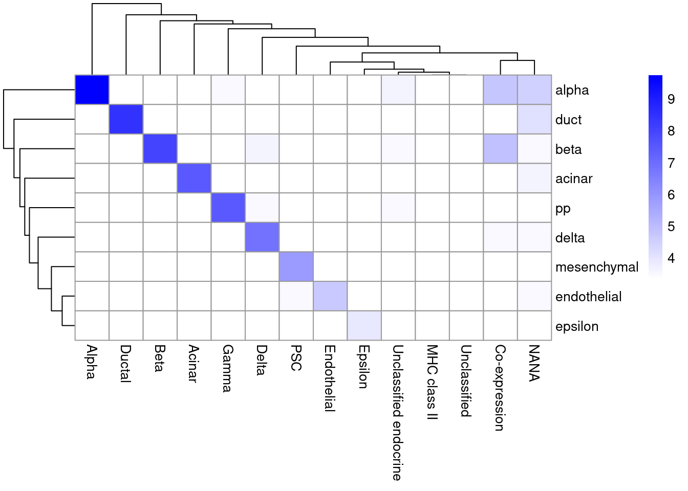
As it so happens, we are in the fortunate position where our test dataset also contains independently defined labels.
We see strong consistency between the two sets of labels (Figure \@ref(fig:singler-comp-pancreas)), indicating that our automatic annotation is comparable to that generated manually by domain experts.
```r
tab <- table(pred.seger$pruned.labels, sce.seger$CellType)
library(pheatmap)
pheatmap(log2(tab+10), color=colorRampPalette(c("white", "blue"))(101))
```
(\#fig:singler-comp-pancreas)Heatmap of the confusion matrix between the predicted labels (rows) and the independently defined labels (columns) in the Segerstolpe dataset. The color is proportinal to the log-transformed number of cells with a given combination of labels from each set.
An interesting question is - given a single-cell reference dataset, is it better to use it directly or convert it to pseudo-bulk values?
A single-cell reference preserves the "shape" of the subpopulation in high-dimensional expression space, potentially yielding more accurate predictions when the differences between labels are subtle (or at least capturing ambiguity more accurately to avoid grossly incorrect predictions).
However, it also requires more computational work to assign each cell in the test dataset.
We refer to the [other book](https://ltla.github.io/SingleRBook/using-single-cell-references.html#pseudo-bulk-aggregation) for more details on how to achieve a compromise between these two concerns.
## Assigning cell labels from gene sets
A related strategy is to explicitly identify sets of marker genes that are highly expressed in each individual cell.
This does not require matching of individual cells to the expression values of the reference dataset, which is faster and more convenient when only the identities of the markers are available.
We demonstrate this approach using neuronal cell type markers derived from the @zeisel2015brain study.
```r
library(scran)
wilcox.z <- pairwiseWilcox(sce.zeisel, sce.zeisel$level1class,
lfc=1, direction="up")
markers.z <- getTopMarkers(wilcox.z$statistics, wilcox.z$pairs,
pairwise=FALSE, n=50)
lengths(markers.z)
```
```
## astrocytes_ependymal endothelial-mural interneurons
## 79 83 118
## microglia oligodendrocytes pyramidal CA1
## 69 81 125
## pyramidal SS
## 149
```
Our test dataset will be another brain scRNA-seq experiment from @tasic2016adult.
```r
library(scRNAseq)
sce.tasic <- TasicBrainData()
sce.tasic
```
```
## class: SingleCellExperiment
## dim: 24058 1809
## metadata(0):
## assays(1): counts
## rownames(24058): 0610005C13Rik 0610007C21Rik ... mt_X57780 tdTomato
## rowData names(0):
## colnames(1809): Calb2_tdTpositive_cell_1 Calb2_tdTpositive_cell_2 ...
## Rbp4_CTX_250ng_2 Trib2_CTX_250ng_1
## colData names(13): sample_title mouse_line ... secondary_type
## aibs_vignette_id
## reducedDimNames(0):
## altExpNames(1): ERCC
```
We use the *[AUCell](https://bioconductor.org/packages/3.12/AUCell)* package to identify marker sets that are highly expressed in each cell.
This method ranks genes by their expression values within each cell and constructs a response curve of the number of genes from each marker set that are present with increasing rank.
It then computes the area under the curve (AUC) for each marker set, quantifying the enrichment of those markers among the most highly expressed genes in that cell.
This is roughly similar to performing a Wilcoxon rank sum test between genes in and outside of the set, but involving only the top ranking genes by expression in each cell.
```r
library(GSEABase)
all.sets <- lapply(names(markers.z), function(x) {
GeneSet(markers.z[[x]], setName=x)
})
all.sets <- GeneSetCollection(all.sets)
library(AUCell)
rankings <- AUCell_buildRankings(counts(sce.tasic),
plotStats=FALSE, verbose=FALSE)
cell.aucs <- AUCell_calcAUC(all.sets, rankings)
results <- t(assay(cell.aucs))
head(results)
```
```
## gene sets
## cells astrocytes_ependymal endothelial-mural interneurons
## Calb2_tdTpositive_cell_1 0.1387 0.04264 0.5306
## Calb2_tdTpositive_cell_2 0.1366 0.04885 0.4538
## Calb2_tdTpositive_cell_3 0.1087 0.07270 0.3459
## Calb2_tdTpositive_cell_4 0.1322 0.04993 0.5113
## Calb2_tdTpositive_cell_5 0.1513 0.07161 0.4930
## Calb2_tdTpositive_cell_6 0.1342 0.09161 0.3378
## gene sets
## cells microglia oligodendrocytes pyramidal CA1
## Calb2_tdTpositive_cell_1 0.04845 0.1318 0.2318
## Calb2_tdTpositive_cell_2 0.02683 0.1211 0.2063
## Calb2_tdTpositive_cell_3 0.03583 0.1567 0.3219
## Calb2_tdTpositive_cell_4 0.05388 0.1481 0.2547
## Calb2_tdTpositive_cell_5 0.06656 0.1386 0.2088
## Calb2_tdTpositive_cell_6 0.03201 0.1553 0.4011
## gene sets
## cells pyramidal SS
## Calb2_tdTpositive_cell_1 0.3477
## Calb2_tdTpositive_cell_2 0.2762
## Calb2_tdTpositive_cell_3 0.5244
## Calb2_tdTpositive_cell_4 0.3506
## Calb2_tdTpositive_cell_5 0.3010
## Calb2_tdTpositive_cell_6 0.5393
```
We assign cell type identity to each cell in the test dataset by taking the marker set with the top AUC as the label for that cell.
Our new labels mostly agree with the original annotation from @tasic2016adult, which is encouraging.
The only exception involves misassignment of oligodendrocyte precursors to astrocytes, which may be understandable given that they are derived from a common lineage.
In the absence of prior annotation, a more general diagnostic check is to compare the assigned labels to cluster identities, under the expectation that most cells of a single cluster would have the same label (or, if multiple labels are present, they should at least represent closely related cell states).
```r
new.labels <- colnames(results)[max.col(results)]
tab <- table(new.labels, sce.tasic$broad_type)
tab
```
```
##
## new.labels Astrocyte Endothelial Cell GABA-ergic Neuron
## astrocytes_ependymal 43 2 0
## endothelial-mural 0 27 0
## interneurons 0 0 759
## microglia 0 0 0
## oligodendrocytes 0 0 1
## pyramidal SS 0 0 1
##
## new.labels Glutamatergic Neuron Microglia Oligodendrocyte
## astrocytes_ependymal 0 0 0
## endothelial-mural 0 0 0
## interneurons 2 0 0
## microglia 0 22 0
## oligodendrocytes 0 0 38
## pyramidal SS 810 0 0
##
## new.labels Oligodendrocyte Precursor Cell Unclassified
## astrocytes_ependymal 20 4
## endothelial-mural 0 2
## interneurons 0 15
## microglia 0 1
## oligodendrocytes 2 0
## pyramidal SS 0 60
```
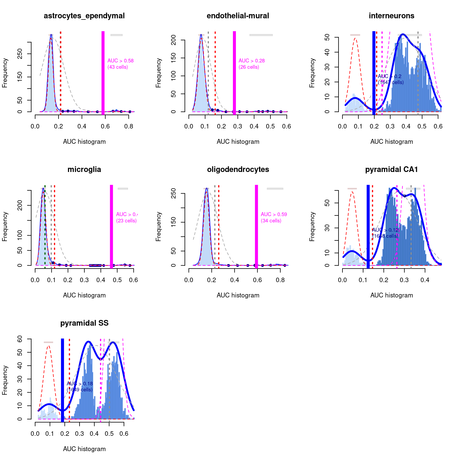
As a diagnostic measure, we examine the distribution of AUCs across cells for each label (Figure \@ref(fig:auc-dist)).
In heterogeneous populations, the distribution for each label should be bimodal with one high-scoring peak containing cells of that cell type and a low-scoring peak containing cells of other types.
The gap between these two peaks can be used to derive a threshold for whether a label is "active" for a particular cell.
(In this case, we simply take the single highest-scoring label per cell as the labels should be mutually exclusive.)
In populations where a particular cell type is expected, lack of clear bimodality for the corresponding label may indicate that its gene set is not sufficiently informative.
```r
par(mfrow=c(3,3))
AUCell_exploreThresholds(cell.aucs, plotHist=TRUE, assign=TRUE)
```
(\#fig:auc-dist)Distribution of AUCs in the Tasic brain dataset for each label in the Zeisel dataset. The blue curve represents the density estimate, the red curve represents a fitted two-component mixture of normals, the pink curve represents a fitted three-component mixture, and the grey curve represents a fitted normal distribution. Vertical lines represent threshold estimates corresponding to each estimate of the distribution.
Interpretation of the *[AUCell](https://bioconductor.org/packages/3.12/AUCell)* results is most straightforward when the marker sets are mutually exclusive, as shown above for the cell type markers.
In other applications, one might consider computing AUCs for gene sets associated with signalling or metabolic pathways.
It is likely that multiple pathways will be active in any given cell, and it is tempting to use the AUCs to quantify this activity for comparison across cells.
However, such comparisons must be interpreted with much caution as the AUCs are competitive values - any increase in one pathway's activity will naturally reduce the AUCs for all other pathways, potentially resulting in spurious differences across the population.
As we mentioned previously, the advantage of the *[AUCell](https://bioconductor.org/packages/3.12/AUCell)* approach is that it does not require reference expression values.
This is particularly useful when dealing with gene sets derived from the literature or other qualitative forms of biological knowledge.
For example, we might instead use single-cell signatures defined from MSigDB, obtained as shown below.
```r
# Downloading the signatures and caching them locally.
library(BiocFileCache)
bfc <- BiocFileCache(ask=FALSE)
scsig.path <- bfcrpath(bfc, file.path("http://software.broadinstitute.org",
"gsea/msigdb/supplemental/scsig.all.v1.0.symbols.gmt"))
scsigs <- getGmt(scsig.path)
```
The flipside is that information on relative expression is lost when only the marker identities are used.
The net effect of ignoring expression values is difficult to predict; for example, it may reduce performance for resolving more subtle cell types, but may also improve performance if the per-cell expression was too noisy to be useful.
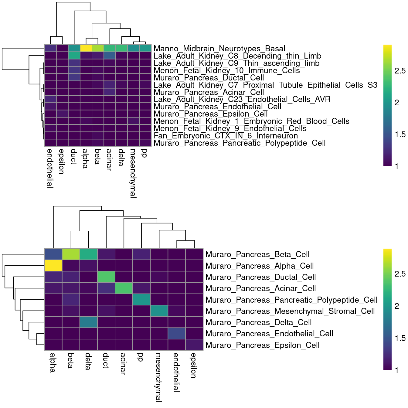
Performance is also highly dependent on the gene sets themselves, which may not be defined in the same context in which they are used.
For example, applying all of the MSigDB signatures on the Muraro dataset is rather disappointing (Figure \@ref(fig:aucell-muraro-heat)), while restricting to the subset of pancreas signatures is more promising.
```r
muraro.mat <- counts(sce.muraro)
rownames(muraro.mat) <- rowData(sce.muraro)$symbol
muraro.rankings <- AUCell_buildRankings(muraro.mat,
plotStats=FALSE, verbose=FALSE)
# Applying MsigDB to the Muraro dataset, because it's human:
scsig.aucs <- AUCell_calcAUC(scsigs, muraro.rankings)
scsig.results <- t(assay(scsig.aucs))
full.labels <- colnames(scsig.results)[max.col(scsig.results)]
tab <- table(full.labels, sce.muraro$label)
fullheat <- pheatmap(log10(tab+10), color=viridis::viridis(100), silent=TRUE)
# Restricting to the subset of Muraro-derived gene sets:
scsigs.sub <- scsigs[grep("Pancreas", names(scsigs))]
sub.aucs <- AUCell_calcAUC(scsigs.sub, muraro.rankings)
sub.results <- t(assay(sub.aucs))
sub.labels <- colnames(sub.results)[max.col(sub.results)]
tab <- table(sub.labels, sce.muraro$label)
subheat <- pheatmap(log10(tab+10), color=viridis::viridis(100), silent=TRUE)
gridExtra::grid.arrange(fullheat[[4]], subheat[[4]])
```
(\#fig:aucell-muraro-heat)Heatmaps of the log-number of cells with each combination of known labels (columns) and assigned MSigDB signatures (rows) in the Muraro data set. The signature assigned to each cell was defined as that with the highest AUC across all (top) or all pancreas-related signatures (bottom).
## Assigning cluster labels from markers
Yet another strategy for annotation is to perform a gene set enrichment analysis on the marker genes defining each cluster.
This identifies the pathways and processes that are (relatively) active in each cluster based on upregulation of the associated genes compared to other clusters.
We demonstrate on the mouse mammary dataset from @bach2017differentiation, using markers that are identified by `findMarkers()` as being upregulated at a log-fold change threshold of 1.
```r
markers.mam <- findMarkers(sce.mam, direction="up", lfc=1)
```
As an example, we obtain annotations for the marker genes that define cluster 2.
We will use gene sets defined by the Gene Ontology (GO) project, which describe a comprehensive range of biological processes and functions.
We define our subset of relevant marker genes at a FDR of 5% and apply the `goana()` function from the *[limma](https://bioconductor.org/packages/3.12/limma)* package.
This performs a hypergeometric test to identify GO terms that are overrepresented in our marker subset.
(The log-fold change threshold mentioned above is useful here, as it avoids including an excessive number of genes from the overpowered nature of per-cell DE comparisons.)
```r
chosen <- "2"
cur.markers <- markers.mam[[chosen]]
is.de <- cur.markers$FDR <= 0.05
summary(is.de)
```
```
## Mode FALSE TRUE
## logical 27819 179
```
```r
# goana() requires Entrez IDs, some of which map to multiple
# symbols - hence the unique() in the call below.
library(org.Mm.eg.db)
entrez.ids <- mapIds(org.Mm.eg.db, keys=rownames(cur.markers),
column="ENTREZID", keytype="SYMBOL")
library(limma)
go.out <- goana(unique(entrez.ids[is.de]), species="Mm",
universe=unique(entrez.ids))
# Only keeping biological process terms that are not overly general.
go.out <- go.out[order(go.out$P.DE),]
go.useful <- go.out[go.out$Ont=="BP" & go.out$N <= 200,]
head(go.useful, 20)
```
```
## Term Ont
## GO:0006641 triglyceride metabolic process BP
## GO:0006639 acylglycerol metabolic process BP
## GO:0006638 neutral lipid metabolic process BP
## GO:0006119 oxidative phosphorylation BP
## GO:0042775 mitochondrial ATP synthesis coupled electron transport BP
## GO:0042773 ATP synthesis coupled electron transport BP
## GO:0046390 ribose phosphate biosynthetic process BP
## GO:0022408 negative regulation of cell-cell adhesion BP
## GO:0009152 purine ribonucleotide biosynthetic process BP
## GO:0035148 tube formation BP
## GO:0022904 respiratory electron transport chain BP
## GO:0009260 ribonucleotide biosynthetic process BP
## GO:0050729 positive regulation of inflammatory response BP
## GO:0022900 electron transport chain BP
## GO:0045333 cellular respiration BP
## GO:0006164 purine nucleotide biosynthetic process BP
## GO:0072522 purine-containing compound biosynthetic process BP
## GO:2001236 regulation of extrinsic apoptotic signaling pathway BP
## GO:0071404 cellular response to low-density lipoprotein particle stimulus BP
## GO:0019432 triglyceride biosynthetic process BP
## N DE P.DE
## GO:0006641 105 11 2.800e-10
## GO:0006639 135 11 4.174e-09
## GO:0006638 137 11 4.876e-09
## GO:0006119 94 9 2.723e-08
## GO:0042775 51 7 8.032e-08
## GO:0042773 52 7 9.226e-08
## GO:0046390 147 10 1.203e-07
## GO:0022408 187 11 1.226e-07
## GO:0009152 131 9 4.818e-07
## GO:0035148 174 10 5.775e-07
## GO:0022904 71 7 8.173e-07
## GO:0009260 140 9 8.443e-07
## GO:0050729 142 9 9.511e-07
## GO:0022900 74 7 1.086e-06
## GO:0045333 145 9 1.133e-06
## GO:0006164 150 9 1.504e-06
## GO:0072522 155 9 1.975e-06
## GO:2001236 163 9 2.992e-06
## GO:0071404 16 4 4.468e-06
## GO:0019432 37 5 6.700e-06
```
We see an enrichment for genes involved in lipid synthesis, cell adhesion and tube formation.
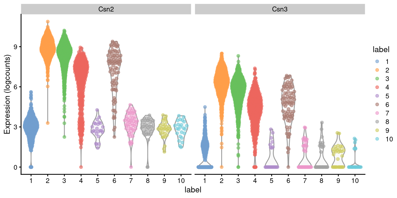
Given that this is a mammary gland experiment, we might guess that cluster 2 contains luminal epithelial cells responsible for milk production and secretion.
Indeed, a closer examination of the marker list indicates that this cluster upregulates milk proteins _Csn2_ and _Csn3_ (Figure \@ref(fig:violin-milk)).
```r
library(scater)
plotExpression(sce.mam, features=c("Csn2", "Csn3"),
x="label", colour_by="label")
```
(\#fig:violin-milk)Distribution of log-expression values for _Csn2_ and _Csn3_ in each cluster.
Further inspection of interesting GO terms is achieved by extracting the relevant genes.
This is usually desirable to confirm that the interpretation of the annotated biological process is appropriate.
Many terms have overlapping gene sets, so a term may only be highly ranked because it shares genes with a more relevant term that represents the active pathway.
```r
# Extract symbols for each GO term; done once.
tab <- select(org.Mm.eg.db, keytype="SYMBOL",
keys=rownames(sce.mam), columns="GOALL")
by.go <- split(tab[,1], tab[,2])
# Identify genes associated with an interesting term.
adhesion <- unique(by.go[["GO:0022408"]])
head(cur.markers[rownames(cur.markers) %in% adhesion,1:4], 10)
```
```
## DataFrame with 10 rows and 4 columns
## Top p.value FDR summary.logFC
##
## Spint2 11 3.28234e-34 1.37163e-31 2.39280
## Epcam 17 8.86978e-94 7.09531e-91 2.32968
## Cebpb 21 6.76957e-16 2.03800e-13 1.80192
## Cd24a 21 3.24195e-33 1.29669e-30 1.72318
## Btn1a1 24 2.16574e-13 6.12488e-11 1.26343
## Cd9 51 1.41373e-11 3.56592e-09 2.73785
## Ceacam1 52 1.66948e-38 7.79034e-36 1.56912
## Sdc4 59 9.15001e-07 1.75467e-04 1.84014
## Anxa1 68 2.58840e-06 4.76777e-04 1.29724
## Cdh1 69 1.73658e-07 3.54897e-05 1.31265
```
Gene set testing of marker lists is a reliable approach for determining if pathways are up- or down-regulated between clusters.
As the top marker genes are simply DEGs, we can directly apply well-established procedures for testing gene enrichment in DEG lists (see [here](https://bioconductor.org/packages/release/BiocViews.html#___GeneSetEnrichment) for relevant packages).
This contrasts with the *[AUCell](https://bioconductor.org/packages/3.12/AUCell)* approach where scores are not easily comparable across cells.
The downside is that all conclusions are made relative to the other clusters, making it more difficult to determine cell identity if an "outgroup" is not present in the same study.
## Computing gene set activities
For the sake of completeness, we should mention that we can also quantify gene set activity on a per-cell level and test for differences in activity.
This inverts the standard gene set testing procedure by combining information across genes first and then testing for differences afterwards.
To avoid the pitfalls mentioned previously for the AUCs, we simply compute the average of the log-expression values across all genes in the set for each cell.
This is less sensitive to the behavior of other genes in that cell (aside from composition biases, as discussed in Chapter \@ref(normalization)).
```r
aggregated <- sumCountsAcrossFeatures(sce.mam, by.go,
exprs_values="logcounts", average=TRUE)
dim(aggregated) # rows are gene sets, columns are cells
```
```
## [1] 22440 2772
```
```r
aggregated[1:10,1:5]
```
```
## [,1] [,2] [,3] [,4] [,5]
## GO:0000002 0.35837 0.3213 0.08054 0.2624 0.2376
## GO:0000003 0.24919 0.2536 0.20097 0.1736 0.2017
## GO:0000009 0.00000 0.0000 0.00000 0.0000 0.0000
## GO:0000010 0.00000 0.0000 0.00000 0.0000 0.0000
## GO:0000012 0.00000 0.1565 0.09245 0.0000 0.2212
## GO:0000014 0.07068 0.2630 0.22187 0.2366 0.3539
## GO:0000015 0.76686 0.4295 0.47544 0.5071 0.8043
## GO:0000016 0.00000 0.0000 0.00000 0.0000 0.0000
## GO:0000017 0.00000 0.0000 0.00000 0.0000 0.6636
## GO:0000018 0.24770 0.2479 0.05839 0.1281 0.1440
```
We can then identify "differential gene set activity" between clusters by looking for significant differences in the per-set averages of the relevant cells.
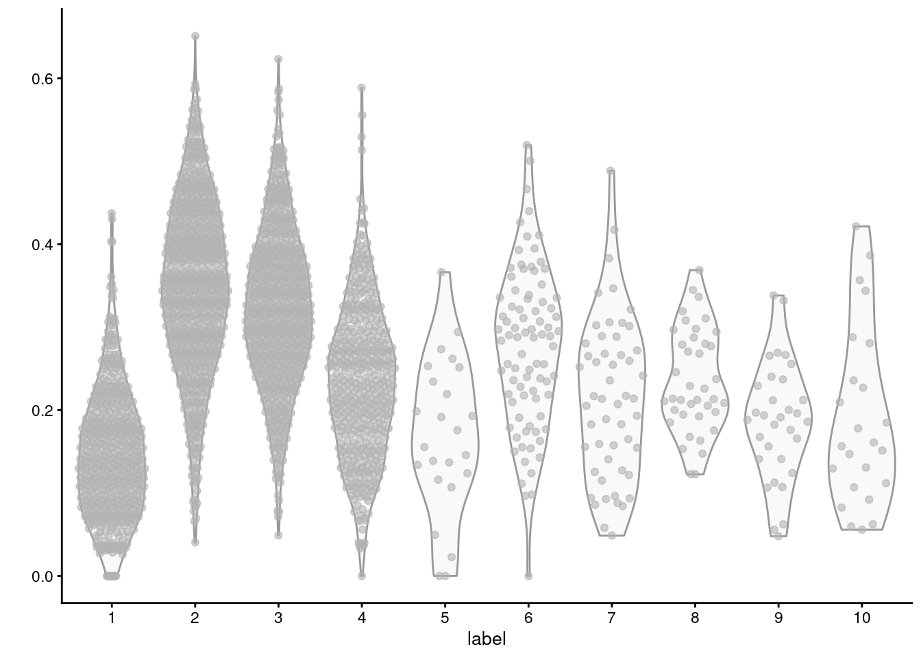
For example, we observe that cluster 2 has the highest average expression for the triacylglycerol biosynthesis GO term (Figure \@ref(fig:lipid-synth-violin)), consistent with the proposed identity of those cells.
```r
plotColData(sce.mam, y=I(aggregated["GO:0019432",]), x="label")
```
(\#fig:lipid-synth-violin)Distribution of average log-normalized expression for genes involved in triacylglycerol biosynthesis, for all cells in each cluster of the mammary gland dataset.
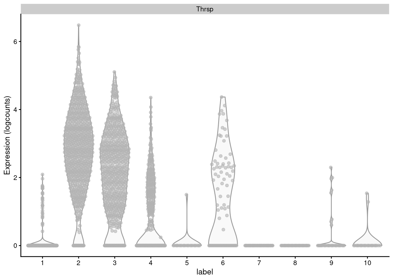
The obvious disadvantage of this approach is that not all genes in the set may exhibit the same pattern of differences.
Non-DE genes will add noise to the per-set average, "diluting" the strength of any differences compared to an analysis that focuses directly on the DE genes (Figure \@ref(fig:thrsp-violin)).
At worst, a gene set may contain subsets of DE genes that change in opposite directions, cancelling out any differences in the per-set average.
This is not uncommon for gene sets that contain both positive and negative regulators of a particular biological process or pathway.
```r
# Choose the top-ranking gene in GO:0019432.
plotExpression(sce.mam, "Thrsp", x="label")
```
(\#fig:thrsp-violin)Distribution of log-normalized expression values for _Thrsp_ across all cells in each cluster of the mammary gland dataset.
We could attempt to use the per-set averages to identify gene sets of interest via differential testing across all possible sets, e.g., with `findMarkers()`.
However, the highest ranking gene sets in this approach tend to be very small and uninteresting because - by definition - the pitfalls mentioned above are avoided when there is only one gene in the set.
This is compounded by the fact that the log-fold changes in the per-set averages are difficult to interpret.
For these reasons, we generally reserve the use of this gene set summary statistic for visualization rather than any real statistical analysis.
## Session Info {-}
![Heatmap of the assignment score for each cell (column) and label (row). Scores are shown before any fine-tuning and are normalized to [0, 1] within each cell.](cell-annotation_files/figure-html/singler-heat-pbmc-1.png)