{width=50%}
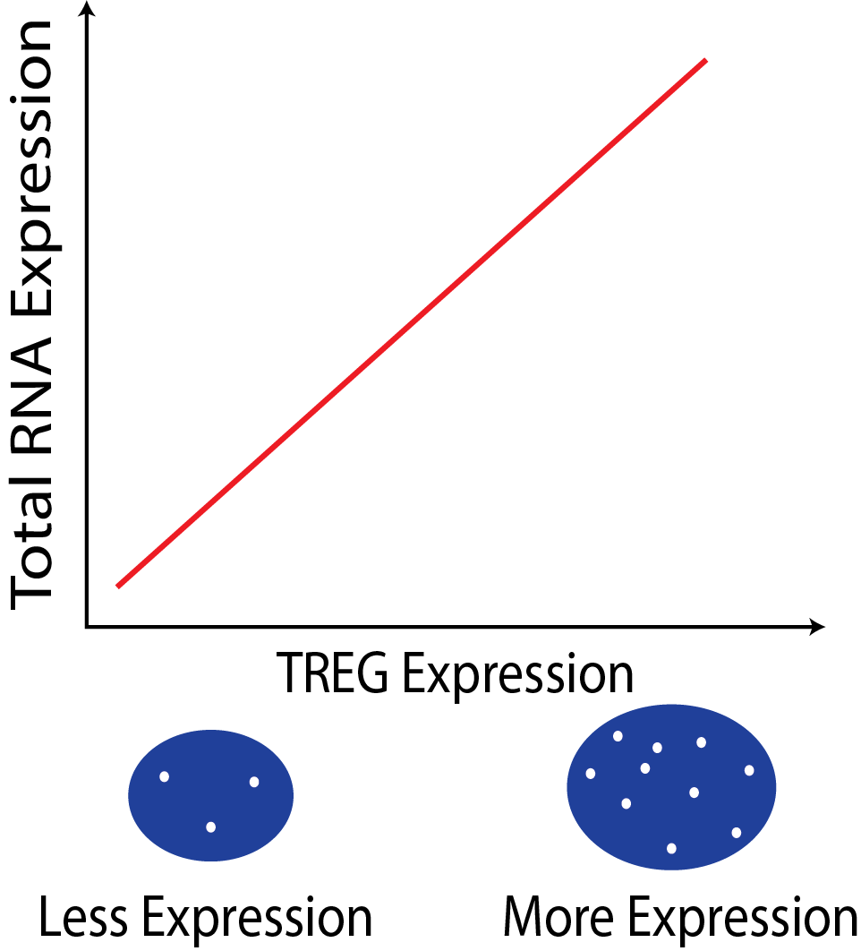
## What makes a gene a good TREG? 1. The gene must have **non-zero expression in most cells** across different tissue and cell types. 2. A TREG should also be expressed at a constant level in respect to other genes across different cell types or have **high rank invariance**. 3. Be **measurable as a continuous metric** in the experimental assay, for example have a dynamic range of puncta when observed in RNAscope. This will need to be considered for the candidate TREGs, and may need to be validated experimentally.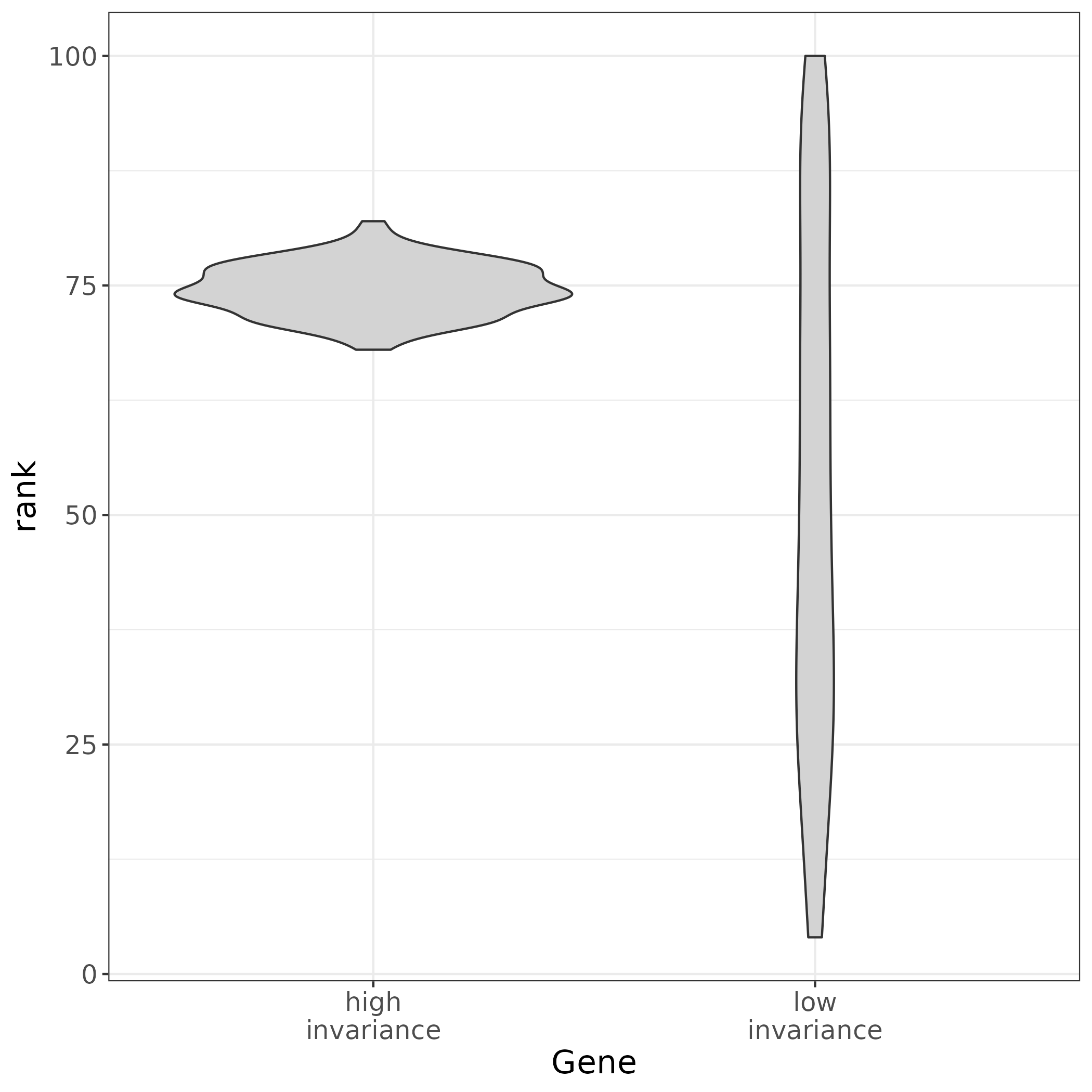{width=30%}
## How to find candidate TREGs with `TREG`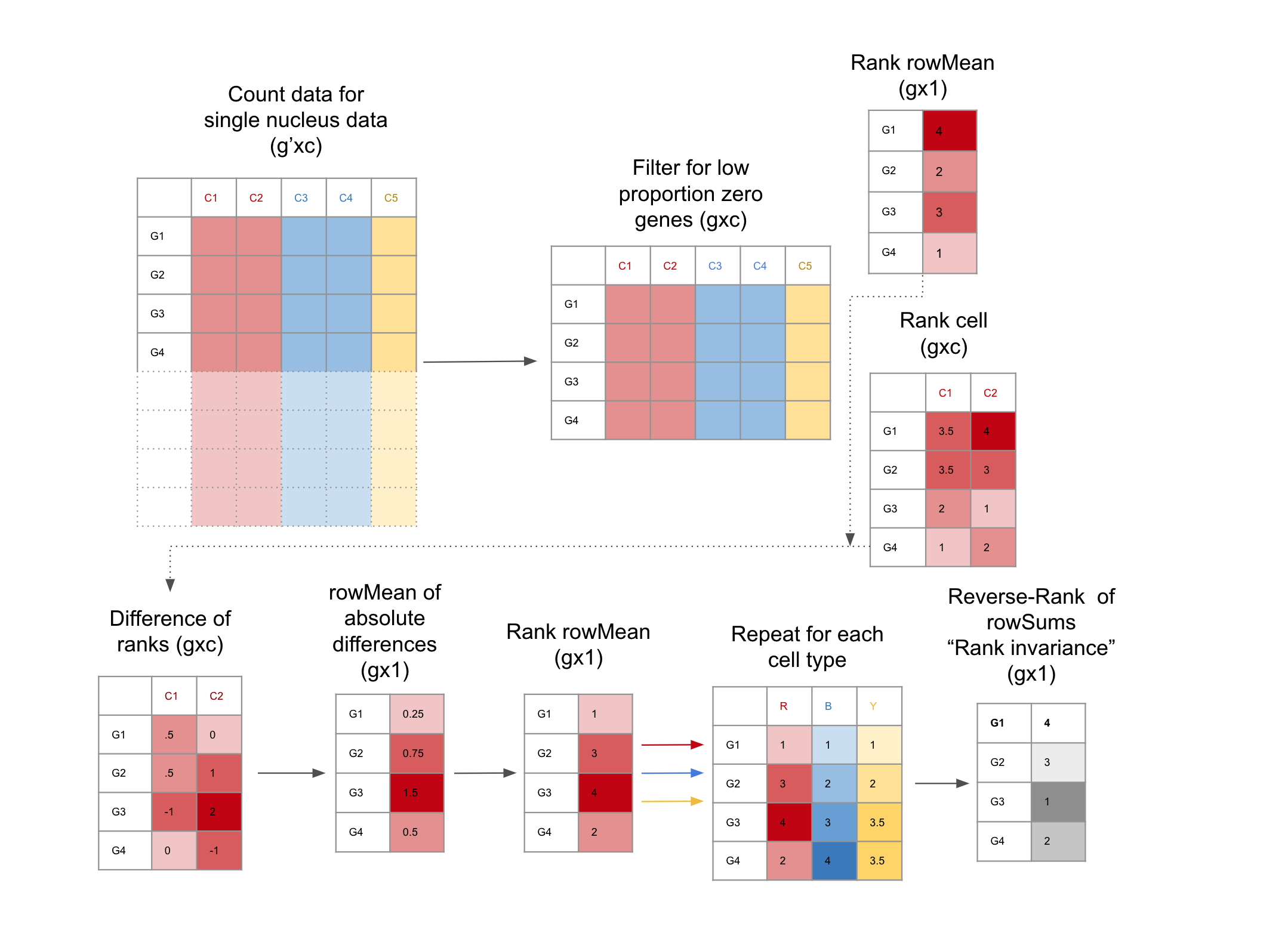{width=100%}
1. **Filter for low Proportion Zero genes snRNA-seq dataset:** This is facilitated with the functions `get_prop_zero()` and `filter_prop_zero()` (Equation \@ref(eq:propZero)). snRNA-seq data is notoriously sparse, these functions enrich for genes with more universal expression. 2. **Evaluate genes for Rank Invariance** The nuclei are grouped only by cell type. Within each cell type, the mean expression for each gene is ranked, the result is a vector (length is the number of genes), using the function `rank_group()`. Then the expression of each gene is ranked for each nucleus,the result is a matrix (the number of nuclei x number of genes), using the function `rank_cells()`.Then the absolute difference between the rank of each nucleus and the mean expression is found, from here the mean of the differences for each gene is calculated, then ranked. These steps are repeated for each group, the result is a matrix of ranks, (number of cell types x number of genes). From here the sum of the ranks for each gene are reversed ranked, so there is one final value for each gene, the “Rank Invariance” The genes with the highest rank-invariance are considered good candidates as TREGs. This is calculated with `rank_invariance_express()`. **This full process is implemented by: `rank_invariance_express()`.** # Example TREG Application In this example we will apply our data driven process for TREG discovery to a snRNA-seq dataset. This process has three main steps: 1. Data prep 2. Gene filtering: dropping genes with low expression and high Proportion Zero (Equation \@ref(eq:propZero)) 3. Rank Invariance Calculation ## Load Packages ```{r "load_packages", message=FALSE, warning=FALSE} library("SingleCellExperiment") library("pheatmap") library("dplyr") library("ggplot2") library("tidyr") library("tibble") ``` ## Download and Prep Data Here we download a public single nucleus RNA-seq (snRNA-seq) data from `r Citep(bib[['tran2021']])` that we'll use as our example. This data can be accessed on [github](https://github.com/LieberInstitute/10xPilot_snRNAseq-human#processed-data). This data is from postmortem human brain in the dorsolateral prefrontal cortex (DLPFC) region, and contains gene expression data for 11k nuclei. We will use `BiocFileCache()` to cache this data. It is stored as a `SingleCellExperiment` object named `sce.dlpfc.tran`, and takes 1.01 GB of RAM memory to load. ```{r "download_DLPFC_data"} # Download and save a local cache of the data available at: # https://github.com/LieberInstitute/10xPilot_snRNAseq-human#processed-data bfc <- BiocFileCache::BiocFileCache() url <- paste0( "https://libd-snrnaseq-pilot.s3.us-east-2.amazonaws.com/", "SCE_DLPFC-n3_tran-etal.rda" ) local_data <- BiocFileCache::bfcrpath(url, x = bfc) load(local_data, verbose = TRUE) ``` ```{r "Data Size Check", echo=FALSE} ## Using 1.01 GB # lobstr::obj_size(sce.dlpfc.tran) ``` ```{r "acronyms", echo=FALSE} ct_names <- tibble( "Cell Type" = c( "Astrocyte", "Excitatory Neurons", "Microglia", "Oligodendrocytes", "Oligodendrocyte Progenitor Cells", "Inhibitory Neurons" ), "Acronym" = c( "Astro", "Excit", "Micro", "Oligo", "OPC", "Inhib" ) ) knitr::kable(ct_names, caption = "Cell type names and corresponding acronyms used in this dataset", label = "acronyms") ``` Human brain tissue consists of many types of cells, for the porpose of this demo, we will focus on the six major cell types listed in Table \@ref(tab:acronyms). ### Filter and Refine to Cell Types of Interest First we will combine all of the Excit, Inhib subtypes, as it is a finer resolution than we want to examine, and combine rare subtypes in to one group. If there are too few cells in a group there may not be enough data to get good results. This new cell type classification is stored in the `colData` as `cellType.broad`. ```{r "define_cell_types"} ## Explore the dimensions and cell type annotations dim(sce.dlpfc.tran) table(sce.dlpfc.tran$cellType) ## Use a lower resolution of cell type annotation sce.dlpfc.tran$cellType.broad <- gsub("_[A-Z]$", "", sce.dlpfc.tran$cellType) (cell_type_tab <- table(sce.dlpfc.tran$cellType.broad)) ``` Next, we will drop any groups with < 50 cells after merging subtypes. This excludes any very rare cell types. Now we are working with the six broad cell types we are interested in. ```{r "drop_small_cell_types"} ## Find cell types with < 50 cells (ct_drop <- names(cell_type_tab)[cell_type_tab < 50]) ## Filter columns of sce object sce.dlpfc.tran <- sce.dlpfc.tran[, !sce.dlpfc.tran$cellType.broad %in% ct_drop] ## Check new cell type bread down and dimension table(sce.dlpfc.tran$cellType.broad) dim(sce.dlpfc.tran) ``` ## Filter Genes Single Nucleus data is often very sparse (lots of zeros in the count data), this dataset is 88% sparse. We can illustrate this in the heat map of the first 1k genes and 500 cells. The heatmap is mostly blue, indicating low values (Figure \@ref(fig:examineSparsity)). ```{r "examineSparsity", fig.cap = "Heatmap of the snRNA-seq counts. Illustrates sparseness of unfiltered data."} ## this data is 88% sparse sum(assays(sce.dlpfc.tran)$counts == 0) / (nrow(sce.dlpfc.tran) * ncol(sce.dlpfc.tran)) ## lets make a heatmap of the first 1k genes and 500 cells count_test <- as.matrix(assays(sce.dlpfc.tran)$logcounts[seq_len(1000), seq_len(500)]) pheatmap(count_test, cluster_rows = FALSE, cluster_cols = FALSE, show_rownames = FALSE, show_colnames = FALSE ) ``` ### Filter to Top 50% Expression Determine the median expression of genes over all rows, drop all the genes that are below this limit. ```{r "top50_filter"} row_means <- rowMeans(assays(sce.dlpfc.tran)$logcounts) (median_row_means <- median(row_means)) sce.dlpfc.tran <- sce.dlpfc.tran[row_means > median_row_means, ] dim(sce.dlpfc.tran) ``` After this filter lets check sparsity and make a heatmap of the first 1k genes and 500 cells. We are seeing more non-blue (Figure \@ref(fig:top50FilterHeatmap))! ```{r "top50FilterHeatmap", fig.cap = "Heatmap of the snRNA-seq counts. With top 50% filtering the data becomes less sparse."} ## this data down to 77% sparse sum(assays(sce.dlpfc.tran)$counts == 0) / (nrow(sce.dlpfc.tran) * ncol(sce.dlpfc.tran)) ## replot heatmap count_test <- as.matrix(assays(sce.dlpfc.tran)$logcounts[seq_len(1000), seq_len(500)]) pheatmap::pheatmap(count_test, cluster_rows = FALSE, cluster_cols = FALSE, show_rownames = FALSE, show_colnames = FALSE ) ``` ### Calculate Proportion Zero and Pick Cutoff For each group (let's use `cellType.broad`) get the Proportion Zero for each gene, where Proportion Zero is defined in Equation \@ref(eq:propZero) where $c_{i,j,k,z}$ is the number of snRNA-seq counts for cell/nucleus $z$ for gene $i$, cell type $j$, brain region $k$, and $n_{j, k}$ is the number of cells/nuclei for cell type $j$ and brain region $k$. \begin{equation} PZ_{i,j,k} = \sum_{z=1}^{n_{j,k}} I(c_{i,j,k} > 0) / n_{j,k} (\#eq:propZero) \end{equation} ```{r "get_prop_zero"} # get prop zero for each gene for each cell type prop_zeros <- get_prop_zero(sce.dlpfc.tran, group_col = "cellType.broad") head(prop_zeros) ``` To determine a good cutoff for filtering lets examine the distribution of these Proportion Zeros by group. ```{r "propZeroDistribution", fig.cap = "Distribution of Proption Zero across cell types and regions."} # Pivot data longer for plotting prop_zero_long <- prop_zeros %>% rownames_to_column("Gene") %>% pivot_longer(!Gene, names_to = "Group", values_to = "prop_zero") # Plot histograms (prop_zero_histogram <- ggplot( data = prop_zero_long, aes(x = prop_zero, fill = Group) ) + geom_histogram(binwidth = 0.05) + facet_wrap(~Group)) ``` Looks like around 0.9 the densities peak, we'll set that as the cutoff (Figure \@ref(fig:propZeroDistribution)). ```{r "pickCutoff", fig.cap = "Show Proportion Zero Cutoff on Distributions."} ## Specify a cutoff, here we use 0.9 propZero_limit <- 0.9 ## Add a vertical red dashed line where the cutoff is located prop_zero_histogram + geom_vline(xintercept = propZero_limit, color = "red", linetype = "dashed") ``` The chosen cutoff excludes the peak Proportion Zeros from all groups (Figure \@ref(fig:pickCutoff)). ### Filter by the Max Proportion Zero Use the cutoff to filter the remaining genes. Only 4k or ~11% of genes pass with this cutoff. Filter the SCE object to this set of genes. ```{r "filter_prop_zero"} ## get a list of filtered genes filtered_genes <- filter_prop_zero(prop_zeros, cutoff = propZero_limit) ## How many genes pass the filter? length(filtered_genes) ## What % of genes is this length(filtered_genes) / nrow(sce.dlpfc.tran) ## Filter the sce object sce.dlpfc.tran <- sce.dlpfc.tran[filtered_genes, ] ``` One last check of the sparsity, more non-blue means more non-zero values for the Rank Invariance calculation, which prevents rank ties (Figure \@ref(fig:propZeroFilterHeatmap)). ```{r "propZeroFilterHeatmap", fig.cap = "Heatmap of the snRNA-seq counts after Proption Zero filtering."} ## this data down to 50% sparse sum(assays(sce.dlpfc.tran)$counts == 0) / (nrow(sce.dlpfc.tran) * ncol(sce.dlpfc.tran)) ## re-plot heatmap count_test <- as.matrix(assays(sce.dlpfc.tran)$logcounts[seq_len(1000), seq_len(500)]) pheatmap::pheatmap(count_test, cluster_rows = FALSE, cluster_cols = FALSE, show_rownames = FALSE, show_colnames = FALSE ) ``` ## Run Rank Invariance To get the Rank Invariance (RI), the rank of the genes across the cells in a group, and between groups is considered. One way to calculate RI is to find the group rank values, and cell rank values separately, then combine them as shown below. The genes with the top RI values are the best candidate TREGs. ```{r "rank_invariance_stepwise"} ## Get the rank of the gene in each group group_rank <- rank_group(sce.dlpfc.tran, group_col = "cellType.broad") ## Get the rank of the gene for each cell cell_rank <- rank_cells(sce.dlpfc.tran, group_col = "cellType.broad") ## Use both rankings to calculate rank_invariance() rank_invar <- rank_invariance(group_rank, cell_rank) ## The top 5 Canidate TREGs: head(sort(rank_invar, decreasing = TRUE)) ``` The `rank_invariance_express()` function combines these three steps into one function, and achieves the same results. ```{r "run_RI_express"} ## rank_invariance_express() runs the previous functions for you rank_invar2 <- rank_invariance_express( sce.dlpfc.tran, group_col = "cellType.broad" ) ## Again the top 5 Canidate TREGs: head(sort(rank_invar2, decreasing = TRUE)) ## Check computationally that the results are identical stopifnot(identical(rank_invar, rank_invar2)) ``` The `rank_invariance_express()` function is more efficient as well, as it loops through the data to rank the genes over cells, and groups at the same time. # Conclusion We have identified top candidate TREG genes from this dataset, by applying Proportion Zero filtering and calculating the Rank Invariance using the `TREG` package. This provides a list of candidate genes that can be useful for estimating total RNA expression in assays such as smFISH. However, we are unable to assess other important qualities of these genes that ensure they are experimentally compatible with the chosen assay. For example, in smFISH with RNAscope it is important that a TREG be expressed at a level that individual puncta can be accurately counted, and have a dynamic range of puncta. During experimental validation we found that _MALAT1_ was too highly expressed in the human DLPFC to segment individual puncta, and ruled it out as an experimentally useful TREG `r Citep(bib[['TREGpaper']])`. Therefore, we recommend that TREGs be evaluated in the assay or analysis of choice you perform a validation experiment with a pilot sample before implementing experiments using it on rare and valuable samples. If you are designing a sc/snRNA-seq study to use as a reference for deconvolution of bulk RNA-seq, we recommend that you generate spatially-adjacent dissections in order to use them for RNAscope experiments. By doing so, you could identify cell types in your sc/snRNA-seq data, then identify candidate TREGs based on those cell types, and use these candidate TREGs in your spatially-adjacent dissections to quantify size and total RNA amounts for the cell types of interest `r Citep(bib[['TREGpaper']])`. Furthermore, the RNAscope data alone can be used as a gold standard reference for cell fractions. TREGs could be useful for other research purposes and other contexts than the ones we envisioned! Thanks for your interest in TREGs :) # Reproducibility The `r Biocpkg('TREG')` package `r Citep(bib[['TREG']])` was made possible thanks to: * R `r Citep(bib[['R']])` * `r Biocpkg('BiocFileCache')` `r Citep(bib[['BiocFileCache']])` * `r Biocpkg('BiocStyle')` `r Citep(bib[['BiocStyle']])` * `r CRANpkg('dplyr')` `r Citep(bib[['dplyr']])` * `r CRANpkg('ggplot2')` `r Citep(bib[['ggplot2']])` * `r CRANpkg('knitr')` `r Citep(bib[['knitr']])` * `r CRANpkg('Matrix')` `r Citep(bib[['Matrix']])` * `r CRANpkg('pheatmap')` `r Citep(bib[['pheatmap']])` * `r CRANpkg('purrr')` `r Citep(bib[['purrr']])` * `r CRANpkg('rafalib')` `r Citep(bib[['rafalib']])` * `r CRANpkg("RefManageR")` `r Citep(bib[["RefManageR"]])` * `r CRANpkg('rmarkdown')` `r Citep(bib[['rmarkdown']])` * `r CRANpkg('sessioninfo')` `r Citep(bib[['sessioninfo']])` * `r Biocpkg('SummarizedExperiment')` `r Citep(bib[['SummarizedExperiment']])` * `r CRANpkg('testthat')` `r Citep(bib[['testthat']])` * `r CRANpkg('tibble')` `r Citep(bib[['tibble']])` * `r CRANpkg('tidyr')` `r Citep(bib[['tidyr']])` Code for creating the vignette ```{r createVignette, eval=FALSE} ## Create the vignette library("rmarkdown") system.time(render("finding_Total_RNA_Expression_Genes.Rmd")) ## Extract the R code library("knitr") knit("finding_Total_RNA_Expression_Genes.Rmd", tangle = TRUE) ``` Date the vignette was generated. ```{r reproduce1, echo=FALSE} ## Date the vignette was generated Sys.time() ``` Wallclock time spent generating the vignette. ```{r reproduce2, echo=FALSE} ## Processing time in seconds totalTime <- diff(c(startTime, Sys.time())) round(totalTime, digits = 3) ``` `R` session information. ```{r reproduce3, echo=FALSE} ## Session info library("sessioninfo") options(width = 120) session_info() ``` # Bibliography This vignette was generated using `r Biocpkg('BiocStyle')` `r Citep(bib[['BiocStyle']])`, `r CRANpkg('knitr')` `r Citep(bib[['knitr']])` and `r CRANpkg('rmarkdown')` `r Citep(bib[['rmarkdown']])` running behind the scenes. Citations made with `r CRANpkg('RefManageR')` `r Citep(bib[['RefManageR']])`. ```{r vignetteBiblio, results = 'asis', echo = FALSE, warning = FALSE, message = FALSE} ## Print bibliography PrintBibliography(bib, .opts = list(hyperlink = "to.doc", style = "html")) ```